library(tidyverse)
library(archive)
library(arrow)
library(RSQLite)
library(tidymodels)
library(butcher)
library(future)
library(tidyfinance) # for portfolio sorts
# install.packages("ranger")
# install.packages("glmnet")
# install.packages("brulee")This blog post is an attempt to replicate the core elements of the paper Empirical Asset Pricing via Machine Learning by Shihao Gu, Brian Kelly, and Dacheng Xiu1. In its essence, the paper presents a horse-race for off-the-shelf machine learning (ML) models to predict return premia. For the replication I often refer to the Online Appendix of the paper, which is available here.
Warning
To render this blog post, I used a virtual machine with 32 CPU cores and 192 GB of memory. Given the dataset I work with is huge, the later may play a major role for replication on your own machine. However, the data-intensive tasks can be split into many smaller tasks, so with minor adjustments everybody should be able to replicate everything I do. I provide some reflections on reducing the computational burden at the end of the blog post.
The code relies on the following R packages. Note that the packages ranger, glmnet, and brulee are only needed if you want to implement the random forests, elastic net, or neural networks, respectively.
Data preparation
Download stock-characteristics
we build a large collection of stock-level predictive characteristics based on the cross-section of stock returns literature. These include 94 characteristics (61 of which are updated annually, 13 are updated quarterly, and 20 are updated monthly). In addition, we include 74 industry dummies corresponding to the first two digits of Standard Industrial Classification (SIC) codes.
The authors provide the dataset with stock-level characteristics online. While the original sample from the published version ended in December 2016, the author furnished the stock-level characteristics dataset until 2021. I download this (large) dataset directly from within R from the Dacheng Xiu’s homepage. The data is stored as a .csv file within a zipped folder. For such purposes, the archive package is useful. I set options(timeout = 1200), which allows the R session to download the dataset for 20 minutes. The default in R is 60 seconds which was too short on my machine.
options(timeout = 1200)
characteristics <- read_csv(archive_read("https://dachxiu.chicagobooth.edu/download/datashare.zip",
                                         file = "datashare.csv"))

characteristics <- characteristics |>
  rename(month = DATE) |>
  mutate(
    month = ymd(month),
    month = floor_date(month, "month")
  ) |>
  rename_with(~ paste0("characteristic_", .),
              -c(permno, month, sic2))

characteristics <- characteristics |>
  drop_na(sic2) |>
  mutate(sic2 = as_factor(sic2))
The characteristics appear in raw format. As many machine-learning applications are sensitive to the scaling of the data, one typically employs some form of standardization.
We cross-sectionally rank all stock characteristics period-by-period and map these ranks into the [-1, 1] interval (footnote 29).
The idea is that at each date, the cross-section of each predictor should be scaled such that the maximum value is 1 and the minimum value is -1. The cross-sectional ranking is time-consuming. The function below explicitly handles NA values, so they do not tamper with the ranking.
rank_transform <- function(x) {
  rank_x <- rank(x)
  rank_x[is.na(x)] <- NA
  min_rank <- 1
  max_rank <- length(na.omit(x))

  if (max_rank == 0) { # only NAs
    return(rep(NA, length(x)))
  } else {
    return(2 * ((rank_x - min_rank) / (max_rank - min_rank) - 0.5))
  }
}

characteristics <- characteristics |>
  group_by(month) |>
  mutate(across(contains("characteristic"), rank_transform)) |>
  ungroup()
Warning
In this blog post I only run code which fits a random forest. Random forests are known for being low-maintenance when it comes to feature engineering and indeed, the transformation and scaling of the predictors does not affect the fitted Random forest. However, as I also show how to fit methods which are sensitive to the scaling of the predictors, I include this crucial part of data preparation.
Another issue is missing characteristics, which we replace with the cross-sectional median at each month for each stock, respectively (footnote 30).
The paper actually claims that each missing value is replaced by the cross-sectional median at each month. However, one of the paper’s coauthors also claims otherwise:
NA values are set to zero (Q&A file furnished by Shihoa Gu)
I interpret the divergence as follows: First, I replace missing values with the cross-sectional median. However, for some months, few characteristics (e.g. absacc) do not have any value at all, leaving the cross-sectional median undefined. Thus, in a second step, I replace remaining missing characteristics with zero.
characteristics <- characteristics |>
  group_by(month) |>
  mutate(across(contains("characteristic"),
                \(x) replace_na(x, median(x, na.rm = TRUE)))) |>
  ungroup()

characteristics <- characteristics |>
  mutate(across(contains("characteristic"),
                \(x) replace_na(x, 0)))
We obtain monthly total individual equity returns from CRSP for all firms listed in the NYSE, AMEX, and NASDAQ. Our sample begins in March 1957 (the start date of the S&P 500) (p. 2248)
To retrieve CRSP excess returns, we merge the stock-level characteristics with the prepared monthly CRSP data as described in WRDS, CRSP, and Compustat. Note that in the book we start the CRSP sample in the year 1960 (partially due to data availability). The difference of three years may explain some deviations in the predictive performance. You can easily adjust the variable start_date <- ymd("1957-03-01") when running the code to reproduce the file tidy_finance_r.sqlite.
To create portfolio sorts based on the predictions, mktcap_lag remains in the sample (albeit it should be mentioned that the main results in Section 2.4.2 of the paper are derived computing equal-weighted portfolios).
We also construct eight macroeconomic predictors following the variable definitions detailed in Welch and Goyal (2008), including dividend-price ratio (dp), earnings-price ratio (ep), book-to-market ratio (bm), net equity expansion (ntis), Treasury-bill rate (tbl), term spread (tms), default spread (dfy), and stock variance (svar). (p. 2248)
We rely on the preparation of the macroeconomic predictors from the corresponding chapter in Accessing and Managing Financial Data. The following code snippets merges the stock-level characteristics with the CRSP sample and the macroeconomic predictors. Note that no further adjustment of the timing of excess returns and stock-level characteristics is necessary:
In this dataset, we’ve already adjusted the lags. (e.g. When DATE=19570329 in our dataset, you can use the monthly RET at 195703 as the response variable.) (readme.txt from the available dataset on Dacheng Xiu’s homepage).
To remain consistent, we only lag the macropredictors by one month.
tidy_finance <- dbConnect(SQLite(),
                          "data/tidy_finance_r.sqlite",
                          extended_types = TRUE)

crsp_monthly <- tbl(tidy_finance, "crsp_monthly") |>
  select(month, permno, mktcap_lag, ret_excess) |>
  collect()

macro_predictors <- tbl(tidy_finance, "macro_predictors") |>
  select(month, dp, ep, bm, ntis, tbl, tms, dfy, svar) |>
  collect() |>
  rename_with(~ paste0("macro_", .), -month)

macro_predictors <- macro_predictors |>
  select(month) |>
  left_join(macro_predictors |> mutate(month = month %m+% months(1)),
            join_by(month))

characteristics <- characteristics |>
  inner_join(crsp_monthly, join_by(month, permno)) |>
  inner_join(macro_predictors, join_by(month)) |>
  arrange(month, permno) |>
  mutate(macro_intercept = 1) |>
  select(permno, month, ret_excess, mktcap_lag,
         sic2, contains("macro"), contains("characteristic"))
Create dataset with all interaction terms
Before applying machine-learning models, the authors include interaction terms between macroeconomic predictors and stock characteristics in the sample.
We include 74 industry dummies corresponding to the first two digits of Standard Industrial Classification (SIC) codes. […] [The stock-level covariates also include] interactions between stock-level characteristics and macroeconomic state variables. The total number of covariates is 94×(8+1)+74=920. (p. 2249)
The following recipe creates dummies for each sic2 code and adds interaction terms between macro variables and stock characteristics. Note that data for the recipe is only required to identify the columns in the sample. No computations are performed at the first step. For that reason, I call head() to keep the computational burden a bit lower without affecting the outcome.
rec <- recipe(ret_excess ~ ., data = characteristics |> head())|>
  update_role(permno, month, mktcap_lag,
              new_role = "id") |>
  step_interact(terms = ~ contains("characteristic"):contains("macro"),
                keep_original_cols = FALSE) |>
  step_dummy(sic2,
             one_hot = TRUE)

rec <- prep(rec)
Next, I create the full dataset containing 3,046,332 monthly observations and 920 covariates.
characteristics_prepared <- bake(rec, new_data = characteristics)I store the prepared file for your convenience. Furthermore, the authors never use the entire dataset for training, instead, only a fraction needs to be available in memory at any given point in time.
characteristics_prepared |>
  group_by(year = year(month)) |>
  write_dataset(path = "data/characteristics_prepared")
Sample splitting and tuning
We divide the 60 years of data into 18 years of training sample (1957–1974), 12 years of validation sample (1975–1986), and the remaining 30 years (1987–2016) for out-of-sample testing. Because machine learning algorithms are computationally intensive, we avoid recursively refitting models each month. Instead, we refit once every year as most of our signals are updated once per year. Each time we refit, we increase the training sample by 1 year. We maintain the same size of the validation sample, but roll it forward to include the most recent 12 months
I visualize my understanding of this data-budget below.
validation_length <- 12

estimation_periods <- tibble(oos_year = 1987:2021,
                             validation_end = oos_year - 1,
                             validation_start = oos_year - validation_length,
                             training_start = 1957,
                             training_end = validation_start - 1) |>
  select(contains("training"), validation_start, validation_end, oos_year)

visualization_data = pmap_dfr(estimation_periods,
                              \(training_start,
                                training_end,
                                validation_start,
                                validation_end,
                                oos_year){
  tibble(year = 1957:2021,
         classification = case_when(year >= training_start & year <= training_end ~ "Training",
                                    year >= validation_start & year <= validation_end ~ "Validation",
                                    year == oos_year ~ "OOS"),
         oos_year)
  }) |>
  drop_na()

ggplot(visualization_data,
       aes(x = year, y = oos_year, color = classification)) +
  geom_point(size = 1) +
  labs(title = "Data classification timeline",
       x = NULL, y = NULL, color = NULL) +
  theme_minimal() +
  theme(axis.text.y = element_blank(),
        axis.ticks.y = element_blank())
Warning: The `scale_name` argument of `discrete_scale()` is deprecated as of
ggplot2 3.5.0.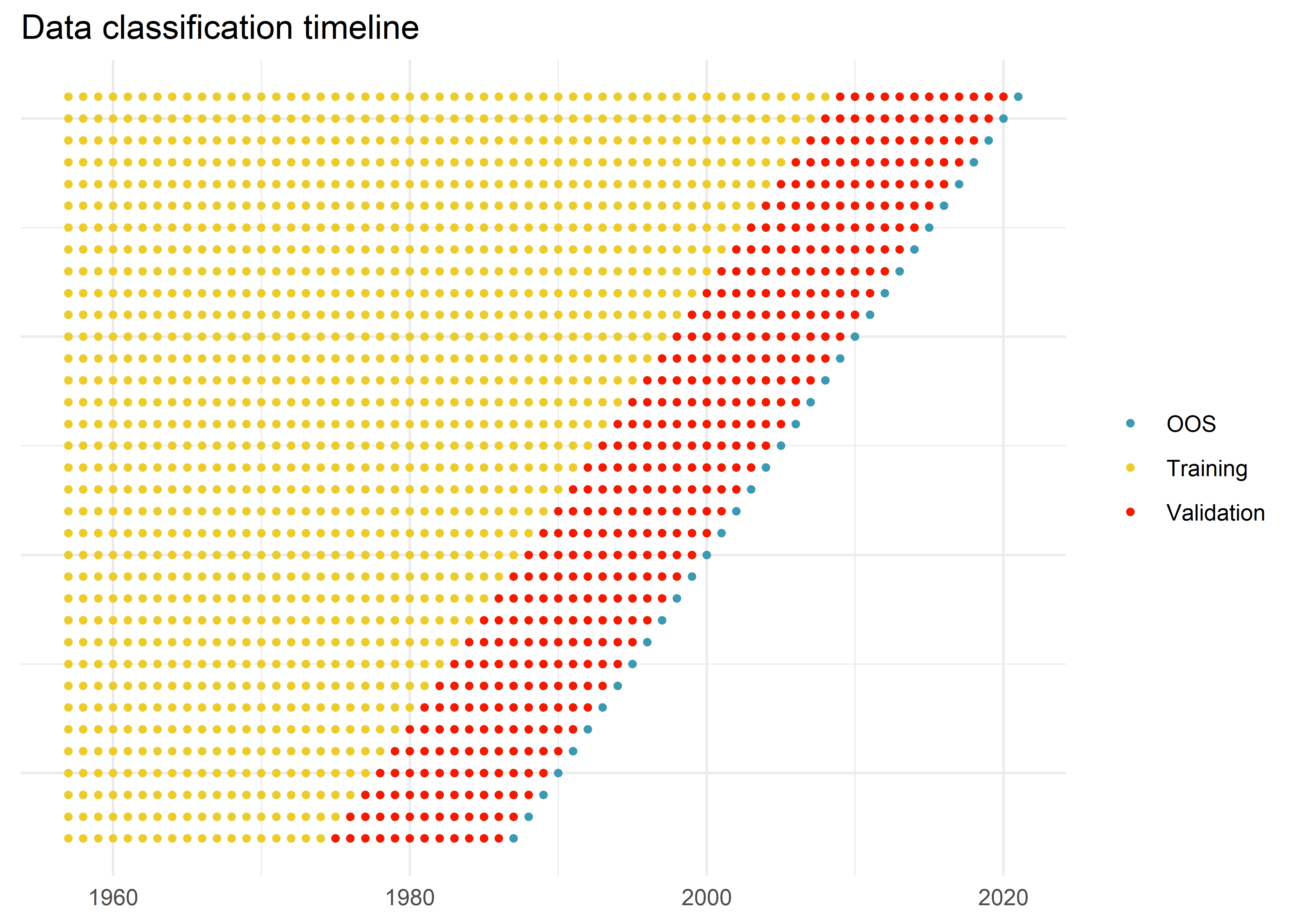
The simple scheme makes model tuning computationally less complex. As there is no need to create several validation sets and thus to reestimate the models several times, the overall time to compute predictions is reduced substantially. One may discuss the substantial sampling variation of the resulting MSPE from the validation sample (typically cross-validation is used to obtain more than one estimate of the prediction error). However, the authors clearly state:
We do not use cross-validation to maintain the temporal ordering of the data. (footnote 32)
Model specification
The paper describes a collection of machine learning methods that was used in the analysis. I refer to Section 1 for a detailed description of the individual models. This blog post focuses on the implementation issues that arise when applying off-the-shelf ML methods on such a large dataset.
characteristics_prepared <- open_dataset(sources = "data/characteristics_prepared")Table A.5 (online appendix) describes the set of hyperparameters and their potential values used for tuning each machine learning model.
In the following I rely on the well-documented tidymodels workflow (e.g. Factor Selection with Machine Learning) to estimate the random forest model.
For the random forest, Table A5 in the Online Appendix states that the number of grown trees is fixed to 300. The number of features in each split is set to \(\in \{3, 5, 10, 20, 30, 50, ...\}\). It is not clear to me what \(...\) means in that context, for that reason I fix the number of choices to six. Finally, in the paper depth is chosen as a hyperparameter, ranging from one (pruned tree) to six (more complex tree). ranger does not support depth as a hyperparameter but rather allows to dynamically stop growing further branches once a minimum number of observations in a group is reached. The effect is similar (if min_n is small, the tree can grow deep, otherwise we expect pruned trees), but cannot be translated directly into depth. I set the option num.threads to allow parallelization for the construction of the trees according to the documentation of the ranger engine in tidymodels.
# install.packages("ranger")

rf_model <- rand_forest(
  mtry = tune(),
  trees = 300,
  min_n = tune()
) |>
  set_engine("ranger",
             num.threads = parallel::detectCores(logical = FALSE) - 1) |>
  set_mode("regression")

rf_grid <- expand_grid(
  mtry = c(3, 5, 10, 20, 30, 50),
  min_n = c(5000, 10000)
)
rec_final <- recipe(ret_excess ~ 0 + .,
data = characteristics_prepared |> head() |> collect()) |>
update_role(permno, month, mktcap_lag, year, new_role = "id")
ml_workflow <- workflow() |>
add_model(rf_model) |>
add_recipe(rec_final)Model fitting
The following performs the model estimation to create predictions for all the years until 2021. For a complete replication of the procedure laid out in the paper, you’ll have to run a loop over all out-of-sample years (j).
j <- 1 # loop until nrow(estimation_periods) for full replication

split_dates <- estimation_periods |>
  filter(row_number() == j)

train <- characteristics_prepared |>
  filter(year(month) < split_dates$training_end) |>
  collect()

validation <- characteristics_prepared |>
  filter(year(month) >= split_dates$validation_start &
           year(month) <= split_dates$validation_end) |>
  collect()

data_split <- make_splits(
  x = train,
  assessment = validation )

folds <- manual_rset(list(data_split),
                     ids = "split")
I tune the model and - after selecting the optimal tuning parameter value based on the prediction error in the validation set - fit the penalized regression using the available data (training and validation test set). The process can be faster by distribution the parameter tuning across multiple workers. tidymodels takes care of this as long as the user specifies a plan. I set the option parallel_over = "resamples" so that the formula is processed only once and then reused across all models that need to be fit. parallelization across the hyperparameter grid in tidymodels is done by initiating a plan() according to the documentation.
plan(multisession, workers = nbrOfWorkers())

ml_fit <- ml_workflow |>
  tune_grid(
    resample = folds,
    grid = rf_grid,
    metrics = metric_set(rmse),
    control = control_grid(parallel_over = "resamples"))
If more computation time is available, it is likely advisable to expand the number of evaluation by providing a wider grid of possible parameter constellations. Next, we finalize the process by selecting the hyperparameter constellation which delivered the smallest mean squared prediction error and fit the model once more using the entire (training and validation) datasets.
ml_fit_best <- ml_fit |>
  select_best(metric = "rmse")

ml_workflow_final <- ml_workflow |>
  finalize_workflow(ml_fit_best) |>
  fit(bind_rows(train, validation))
Trained workflows contain a lot of information which may be redundant for the task at hand: generating predictions. The butcher package provides tooling to “axe” parts of the fitted output that are no longer needed, without sacrificing prediction functionality from the original model object. To provide an intermediary anchor (also to ensure reprocudibility), I follow this example to store the trained model. Julia Silge provided some reflections on best practices here which I tried to incorporate.
fitted_workflow <- butcher(ml_workflow_final)
write_rds(fitted_workflow, file = paste0("data/fitted_workflow_",split_dates$oos_year,".rds"))
Other ML models
While this blog post only shows how to implement the prediction procedure based on the random forest, it is no problem to generate predictions for the remaining main methods (elastic net, neural networks, …) presented in the original paper. Below, I provide code for models that come as close as possible to the specifications laid out in the Online Appendix of the paper.
For OLS, ENet, GLM, and GBRT, we present their robust versions using Huber loss, which perform better than the version without. (p. 2250)
For the sake of simplicity, I only show how to fit linear models using \(l2\) loss functions. In R, the package hqreg implements algorithms for fitting regularization paths for Lasso or elastic net penalized regression models with Huber loss. However, hqreg is not a running engine for pairsnip (yet).
For instance, to fit the elastic net it seems necessary to evaluate the mean-squared prediction error in the validation sample for only two values of the penalty term. Instead of tuning the elastic net mixture coefficient, I follow the paper and show how to fix its value to \(0.5\).
# install.packages("glmnet")

elastic_net <- linear_reg(
  penalty = tune(),
  mixture = 0.5
) |>
  set_engine("glmnet")

penalty_grid = tibble(penalty = c(1e-4, 1e-1))
For the neural network, the paper specifies the manifold architecture choices
Our shallowest neural network has a single hidden layer of 32 neurons, which we denoted NN1. Next, NN2 has two hidden layers with 32 and 16 neurons, respectively; NN3 has three hidden layers with 32, 16, and 8 neurons, respectively; NN4 has four hidden layers with 32, 16, 8, and 4 neurons, respectively; and NN5 has five hidden layers with 32, 16, 8, 4, and 2 neurons, respectively. (p. 2244)
We use the same activation function at all nodes, and choose a popular functional form in recent literature known as the rectified linear unit (ReLU) (p. 2244)
In the following I show the exemplary implementation of the neural network with two hidden layers using the package brulee. Most information is taken from Table A5 in the online appendix. The table mentions a parameter patience = 5 which I understand as a command on how many iterations with no improvement before stopping the optimization process.
# install.packages("brulee")

deep_nnet_model <- mlp(
  epochs = 100,
  hidden_units = c(32, 16),
  activation = "relu",
  learn_rate = tune(),
  penalty = tune(),
  batch_size = 10000,
  stop_iter = 5
) |>
  set_mode("regression") |>
  set_engine("brulee")

nn_grid <- expand_grid(
  learn_rate = c(0.001, 0.01),
  penalty = c(1e-5, 1e-3)
)
Machine-learning portfolios
After fitting the model(s), there are plenty ways to evaluate the predictive performance. In the remainder of the blog post I focus on the economically most meaningful (imho) application presented in the paper:
At the end of each month, we calculate 1-month-ahead out-of-sample stock return predictions for each method. We then sort stocks into deciles based on each model’s forecasts. We reconstitute portfolios each month using value weights. Finally, we construct a zero-net-investment portfolio that buys the highest expected return stocks (decile 10) and sells the lowest (decile 1). (p. 2264)
The following code chunks performs the predictions for every out-of-sample year (starting from 1987): First, I predict stock excess returns based on the fitted model, then we sort assets into portfolios based on the prediction. In line with the original paper, I chose an equal-weighted scheme which is arguably more sensitive to trading cost (see the discussion on p. 2265 of the paper). Note that in the original paper, the model parameters are updated each year.
fitted_workflow <- read_rds("data/fitted_workflow_1987.rds")

create_predictions <- function(oos_year){

  out_of_sample <- characteristics_prepared |>
    filter(year(month) == oos_year) |>
    collect()

  #fitted_workflow <- read_rds(paste0("data/fitted_workflow_", oos_year,".rds"))

  out_of_sample_predictions <- fitted_workflow |>
    predict(out_of_sample)

 out_of_sample <- out_of_sample |>
    select(permno, month, mktcap_lag, ret_excess) |>
    bind_cols(out_of_sample_predictions)

return(out_of_sample)
}


oos_predictions <- estimation_periods |>
  pull(oos_year) |>
  map_dfr(\(x) create_predictions(x))
Warning
Note that I am calling the fitted model from the first out-of-sample year (1987) in each iteration. In other words, the model parameters do not get updated every year as in the original paper. If you estimated the model for each value of \(j\) as described above, you can replace the line above to replicate the original procedure.
To assign portfolios using the predictions, I use the assign_portfolio() from the tidyfinance package.
ml_portfolios <- oos_predictions |>
  group_by(month) |>
  mutate(
    portfolio = assign_portfolio(
      data = pick(everything()),
      sorting_variable = ".pred",
      breakpoint_options(n_portfolios = 10)
    ),
    portfolio = as.factor(portfolio)
  ) |>
  group_by(portfolio, month) |>
  summarize(
    ret_predicted = mean(.pred),
    ret_excess = mean(ret_excess),
    .groups = "drop"
  )
Finally, we evaluate the performance of the ML-portfolios. The table reports the predicted return, the average realized return, the standard deviation, and the out-of-sample Sharpe ratio for each of the decile portfolios as well as the long-short zero-cost portfolio.
hml_portfolio <- ml_portfolios |>
  reframe(
    ret_excess = ret_excess[portfolio == 10] - ret_excess[portfolio == 1],
    ret_predicted = ret_predicted[portfolio == 10] - ret_predicted[portfolio == 1],
    month = month[portfolio == 10],
    portfolio = factor("H-L", levels = as.character(c(1:10, "H-L"))),
  )

ml_portfolios |>
  bind_rows(hml_portfolio) |>
  group_by(portfolio) |>
  summarize(predicted_mean = mean(ret_predicted),
            realized_mean = mean(ret_excess),
            realized_sd = sd(ret_excess),
            sharpe_ratio = realized_mean / realized_sd) |>
  print(n = Inf)
# A tibble: 11 × 5
portfolio predicted_mean realized_mean realized_sd sharpe_ratio
<fct> <dbl> <dbl> <dbl> <dbl>
1 1 -0.0516 -0.162 0.105 -1.54
2 2 -0.0287 -0.126 0.0808 -1.55
3 3 -0.0181 -0.0977 0.0814 -1.20
4 4 -0.0111 -0.0639 0.0672 -0.950
5 5 -0.00558 -0.0350 0.0534 -0.655
6 6 -0.000535 -0.00536 0.0462 -0.116
7 7 0.00447 0.0222 0.0504 0.441
8 8 0.0101 0.0502 0.0688 0.730
9 9 0.0165 0.0849 0.0977 0.870
10 10 0.0290 0.198 0.218 0.909
11 H-L 0.0805 0.360 0.168 2.14 Obviously, the paper is doing much more. In particular, the debate on “which covariates matter” is interesting and not necessarily trivial to implement. However, covering even more goes beyond the scope of a simple blog post. I hope that the code base above helps to overcome any issues with implementing the more intriguing parts of the paper.
Some comments on parallelization
Arguably, the dataset used for this application is huge. So is the computational effort to train the ML methods. Even though I have substantial computing power available, I decided to keep the computational burden limited in the interest of simplicity and time. Should you not have a supercomputer available, the following tipps may help:
- When expanding the characteristics to include all interaction terms by applying the recipe (
bake()), you do not have to use the entire dataset in memory as I do above. It seems plausible to store the characteristics (e.g., inparquetform) and applybake()to each year individually before storing the data year-by-year. The all-in procedure from above requires around 140GB in memory which can be reduced to \(\approx 140/60\) when applying the recipe on an annual basis. - In the blog post, I only fit the random forest for one single year (
j = 1, the first of the 35 out-of-sample periods). It is straightforward to loop overj, starting from 1 until 35 and to store the predictions individually for each year.
- Tuning the model for one out-of-sample period like above is still going to be computational heavy, and I am afraid there is no way around that. For the final out-of-sample period 2021, the training set contains more than two million rows with 920 columns as the set of predictors. The only way I can imagine to reduce the computational burden and still retain some (hopefully) useful predictions is to pre-select a well-balanced set of firms from the CRSP sample which differ with respect to some firm characteristics, e.g. by sampling from the well-known size and book-to-market double sort decile groups.
Footnotes
The Review of Financial Studies, Volume 33, Issue 5, May 2020, Pages 2223–2273, https://doi.org/10.1093/rfs/hhaa009↩︎