Recommender systems are a key component of our digital lifes, ranging from e-commerce, online advertisements, movie recommendations, or more generally all kinds of product recommendations. A recommender system aims to efficiently deliver personalized content to users based on a large pool of potentially relevant information. In this blog post, I illustrate the concept of recommender systems by building a simple stock recommendation tool that relies on publicly available portfolios from the social trading platform wikifolio.com. The resulting recommender proposes stocks to investors who already have their own portfolios and look for new investment opportunities. The underlying assumption is that the wikifolio traders hold stock portfolios that can provide meaningful inspiration for other investors. The resulting stock recommendations of course do not constitute any investment advice and rather serve an illustrative purpose.

wikifolio.com is the leading social trading platform in Europe, where anyone can publish and monetize their trading strategies through virtual portfolios, which are called wikifolios. The community of wikifolio traders includes full time investors and successful entrepreneurs, as well as experts from different sectors, portfolio managers, and editors of financial magazines. All traders share their trading ideas through fully transparent wikifolios. The wikifolios are easy to track and replicate, by investing in the corresponding, collateralized index certificate. As of writing, there are more than 30k published wikifolios of more than 9k traders, indicating a large diversity of available portfolios for training our recommender.

There are essentially three types of recommender models: recommenders via collaborative filtering, recommenders via content-based filtering, and hybrid recommenders (that mix the first two). In this blog post, I focus on the collaborative filtering approach as it requires no information other than portfolios and can provide fairly high precision with little complexity. Nonetheless, I first briefly describe the recommender approaches and refer to Ricci et al. (2011)¹ for a comprehensive exposition.

A Primer on Recommender Systems

Collaborative Filtering

In collaborative filtering, recommendations are based on past user interactions and items to produce new recommendations. The central notion is that past user-item interactions are sufficient to detect similar users or items. Broadly speaking, there are two sub-classes of collaborative filtering: the memory-based approach, which essentially searches nearest neighbors based on recorded transactions and is hence model-free, and the model-based approach, where new representations of users and items are built based on some generative pre-estimated model. Theoretically, the memory-based approach has a low bias (since no latent model is assumed) but a high variance (since the recommendations change a lot in the nearest neighbor search). The model-based approach relies on a trained interaction model. It has a relatively higher bias but a lower variance, i.e., recommendations are more stable since they come from a model.

Advantages of collaborative filtering include: (i) no information about users or items is required; (ii) a high precision can be achieved with little data; (iii) the more interaction between users and items is available, the more recommendations become accurate. However, the disadvantages of collaborative filtering are: (i) it is impossible to make recommendations to a new user or recommend a new item (cold start problem); (ii) calculating recommendations for millions of users or items consumes a lot of computational power (scalability problem); (iii) if the number of items is large relative to the users and most users only have interacted with a small subset of all items, then the resulting representation has many zero interactions and might hence lead to computational difficulties (sparsity problem).

Content-Based Filering

Content-based filtering methods exploit information about users or items to create recommendations by building a model that relates available characteristics of users or items to each other. The recommendation problem is hence cast into a classification problem (the user will like the item or not) or more generally a regression problem (which rating will the user give an item). The classification problem can be item-centered by focusing on available user information and estimating a model for each item. If there are a lot of user-item interactions available, the resulting model is fairly robust, but it is less personalized (as it ignores user characteristics apart from interactions). The classification problem can also be user-centered by working with item features and estimating a model for each user. However, if a user only has a few interactions then the resulting model becomes easily unstable. Content-based filtering can also be neither user nor item-centered by stacking the two feature vectors, hence considering both input simultaneously, and putting them into a neural network.

The main advantage of content-based filtering is that it can make recommendations for new users without any interaction history or recommend new items to users. The disadvantages include: (i) training needs a lot of users and item examples for reliable results; (ii) tuning might be much harder in practice than collaborative filtering; (iii) missing information might be a problem since there is no clear solution how to treat missingness in user or item characteristics.

Hybrid Recommenders

Hybrid recommender systems combine both collaborative and content-based filtering to overcome the challenges of each approach. There are different hybridization techniques available, e.g., combining the scores of different components (weighted), chosing among different component (switching), following strict priority rules (cascading), presenting outputs from different components at the same time (mixed), etc.

Train Collaborative Filtering Recommenders in R

For this post, we rely on the tidyverse (Wickham et al. 2019) family of packages, scales (Wickham and Seidel 2022) for scale functions for visualization, and recommenderlab² - a package that provides an infrastructure to develop and test collaborative filtering recommender algorithms.

library(tidyverse)
library(scales)
library(recommenderlab)

I load a data set with stock holdings of investable wikifolios at the beginning of 2023 that I host in one of my repositories. The data contains the portfolios of 6,544 wikifolios that held in total 5,069 stocks on January 1st 2023.

wikifolio_portfolios <- read_csv("https://raw.githubusercontent.com/christophscheuch/christophscheuch.github.io/main/data/wikifolio_portfolios.csv") 
glimpse(wikifolio_portfolios)

Rows: 149,916
Columns: 2
$ wikifolio <chr> "DE000LS9AAB3", "DE000LS9AAB3", "DE000LS9AAB3", "…
$ stock     <chr> "AU000000CSL8", "AU0000193666", "CA0679011084", "…

First, I convert the long data to a binary rating matrix.

binary_rating_matrix <- wikifolio_portfolios |>
  mutate(in_portfolio = 1) |> 
  pivot_wider(id_cols = wikifolio,
              names_from = stock,
              values_from = in_portfolio,
              values_fill = list(in_portfolio = 0)) |>
  select(-wikifolio) |>
  as.matrix() |>
  as("binaryRatingMatrix")
binary_rating_matrix

6544 x 5069 rating matrix of class 'binaryRatingMatrix' with 149916 ratings.

As in our book chapter on Factor Selection via Machine Learning, I perform cross-validation and split the data into training and test data. The training sample constitute 80% of the data and I perform 5-fold cross validation. Testing is performed by withholding items from the test portfolios (parameter given) and checking how well the algorithm predicts the withheld items. The value given=-1 means that an algorithm sees all but 1 withheld stock for the test portfolios and needs to predict the missing stock. I refer to Breese et al. (1998)³ for a discussion of other withholding strategies.

scheme <- binary_rating_matrix |>
  evaluationScheme(
    method = "cross-validation",
    k      = 5,
    train  = 0.8,
    given  = -1
)
scheme

Evaluation scheme using all-but-1 items
Method: 'cross-validation' with 5 run(s).
Good ratings: NA
Data set: 6544 x 5069 rating matrix of class 'binaryRatingMatrix' with 149916 ratings.

Here is the list of recommenders that I consider for the backtest with some intuition:

Random Items: the benchmark case because it just stupidly chooses random stocks from all possible choices.
Popular Items: just recommends the most popular stocks to measured by the number of wikifolios that hold the stock.
Association Rules: each wikifolio and its portfolio is considered as a transaction. Association rule mining finds similar portfolios across all traders (if traders have x, y and z in their portfolio, then they are X% likely of also including w).
Item-Based Filtering: the algorithm calculates a similarity matrix across stocks. Recommendations are then based on the list of most similar stocks to the ones the wikifolio already has in its portfolio.
User-Based Filtering: the algorithm finds a neighborhood of similar wikifolios for each wikifolio (for this exercise it is set to 100 most similar wikifolios). Recommendations are then based on what the most similar wikifolios have in their portfolio.

For each algorithm, I base the evaluation on 1, 3, 5, and 10 recommendations. This specification means that each algorithm proposes 1 to 10 recommendations to the test portfolios and the evaluation scheme then checks whether the proposals contain the one withheld stock. Note that the evaluation takes a couple of hours, in particular because the Item-Based and User-Based Filtering approaches are quite time-consuming.

algorithms <- list(
  "Random Items"         = list(name  = "RANDOM",  param = NULL),
  "Popular Items"        = list(name  = "POPULAR", param = NULL),
  "Association Rules"    = list(name  = "AR", param = list(supp = 0.01, conf = 0.1)),
  "Item-Based Filtering" = list(name  = "IBCF", param = list(k = 10)),
  "User-Based Filtering" = list(name  = "UBCF", param = list(method = "Cosine", nn = 100))
)

number_of_recommendations <- c(1, 3, 5, 10)
results <- evaluate(
  scheme,
  algorithms,
  type = "topNList",
  progress = TRUE,
  n = number_of_recommendations
)

Evaluate Recommenders

The output of evaluate() already provides the evaluation metrics in a structured way. I can simply average the metrics over the cross-validation folds.

results_tbl <- results |>
  avg() |>
  map(as_tibble) |>
  bind_rows(.id = "model")

Now, for each recommender, we are interested the following numbers:

True Negative (TN) = number of not predicted items that do not correspond to withheld items
False Positive (FP) = number of incorrect predictions that do not correspond to withheld items
False negative (FN) = number of not predicted items that correspond to withheld items
True Positive (TP) = number of correct predictions that correspond to withheld items

The two figures below present the most common evaluation techniques for the performance of recommender algorithms in backtest settings like mine.

ROC curves

The first visualization approach comes from signal-detection and is called “Receiver Operating Characteristic” (ROC). The ROC-curve plots the algorithm’s probability of detection (TPR) against the probability of false alarm (FPR).

TPR = TP / (TP + FN) (i.e., share of true positive recommendations relative to all known portfolios)
FPR = FP / (FP + TN) (i.e., share of incorrect recommendations relative to )

Intuitively, the bigger the area under the ROC curve, the better is the corresponding algorithm.

results_tbl |>
  ggplot(aes(FPR, TPR, colour = model)) +
  geom_line() +
  geom_label(aes(label = n))  +
  labs(
    x = "False Positive Rate (FPR)",
    y = "True Positive Rate (TPR)",
    title = "ROC curves of stock recommender algorithms",
    colour = "Model"
  ) +
  theme(legend.position = "right") + 
  scale_y_continuous(labels = percent) +
  scale_x_continuous(labels = percent)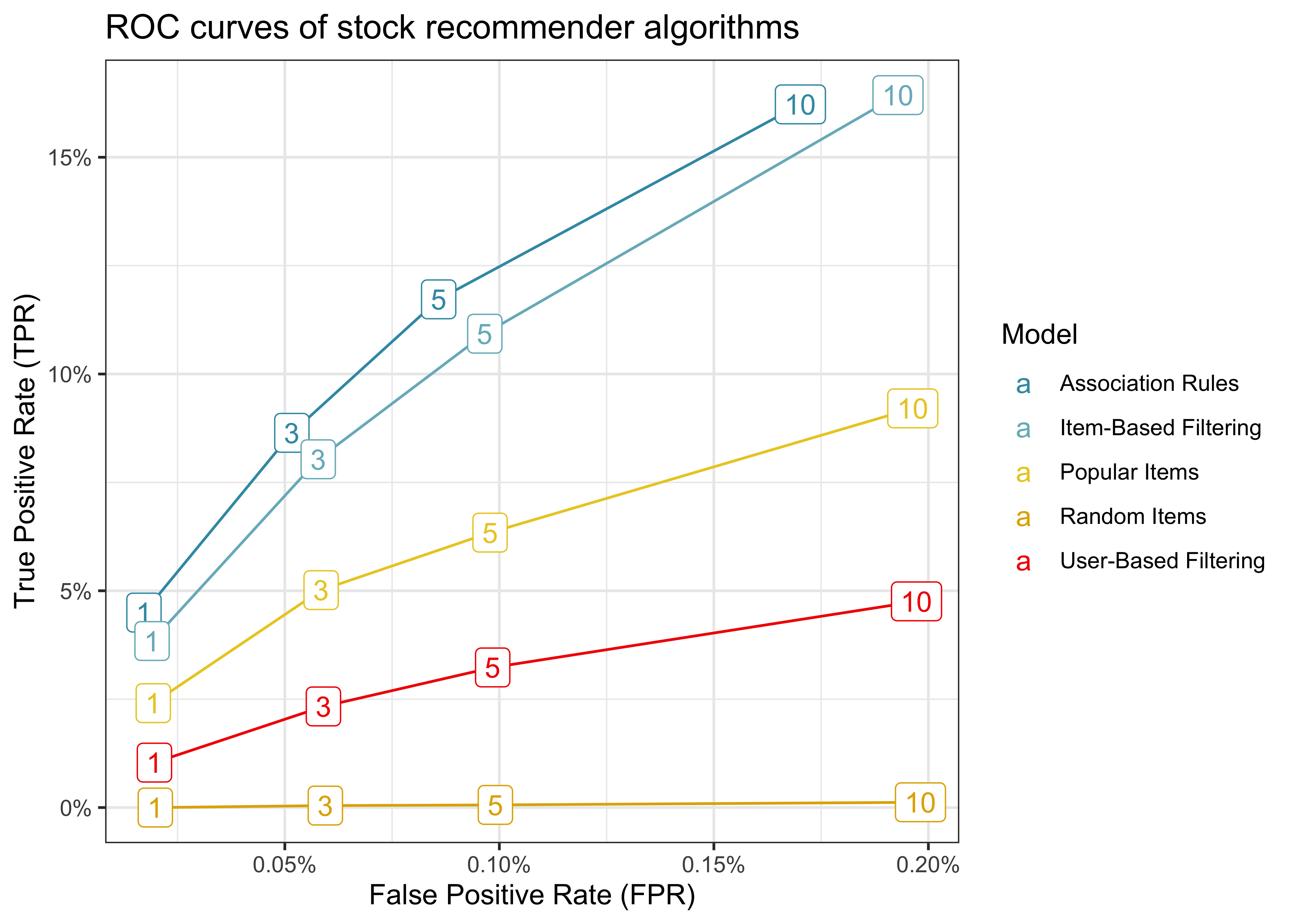

Title: ROC curves of stock recommender algorithms. The figure shows that the association rules mining algorithm achieves the highest true positive rate for any false positive rate.

The figure shows that recommending random items exhibits the lowest TPR for any FPR, so it is the worst among all algorithms (which is not surprising). Association rules, on the other hand, constitute the best algorithm among the current selection. This result is neat because association rule mining is a computationally cheap algorithm, so we could potentially fine-tune or reestimate the model easily.

Precision-Recall Curves

The second popular approach is to plot Precision-Recall curves. The two measures are often used in information retrieval problems:

Precision = TP / (TP + FP) (i.e., correctly recommended items relative to total recommended items)
Recall = TP / (TP + FN) (i.e., correctly recommended items relative to total number of known useful recommendations)

The goal is to have a higher precision for any level of recall. In fact, there is trade-off between the two measures since high precision means low recall and vice-versa.

results_tbl |>
  ggplot(aes(x = recall, y = precision, colour = model)) +
  geom_line() +
  geom_label(aes(label = n))  +
  labs(
    x = "Recall", y = "Precision",
    title = "Precision-Recall curves of stock recommender algorithms",
    colour = "Model"
  ) +
  theme(legend.position = "right") + 
  scale_y_continuous(labels = percent) +
  scale_x_continuous(labels = percent)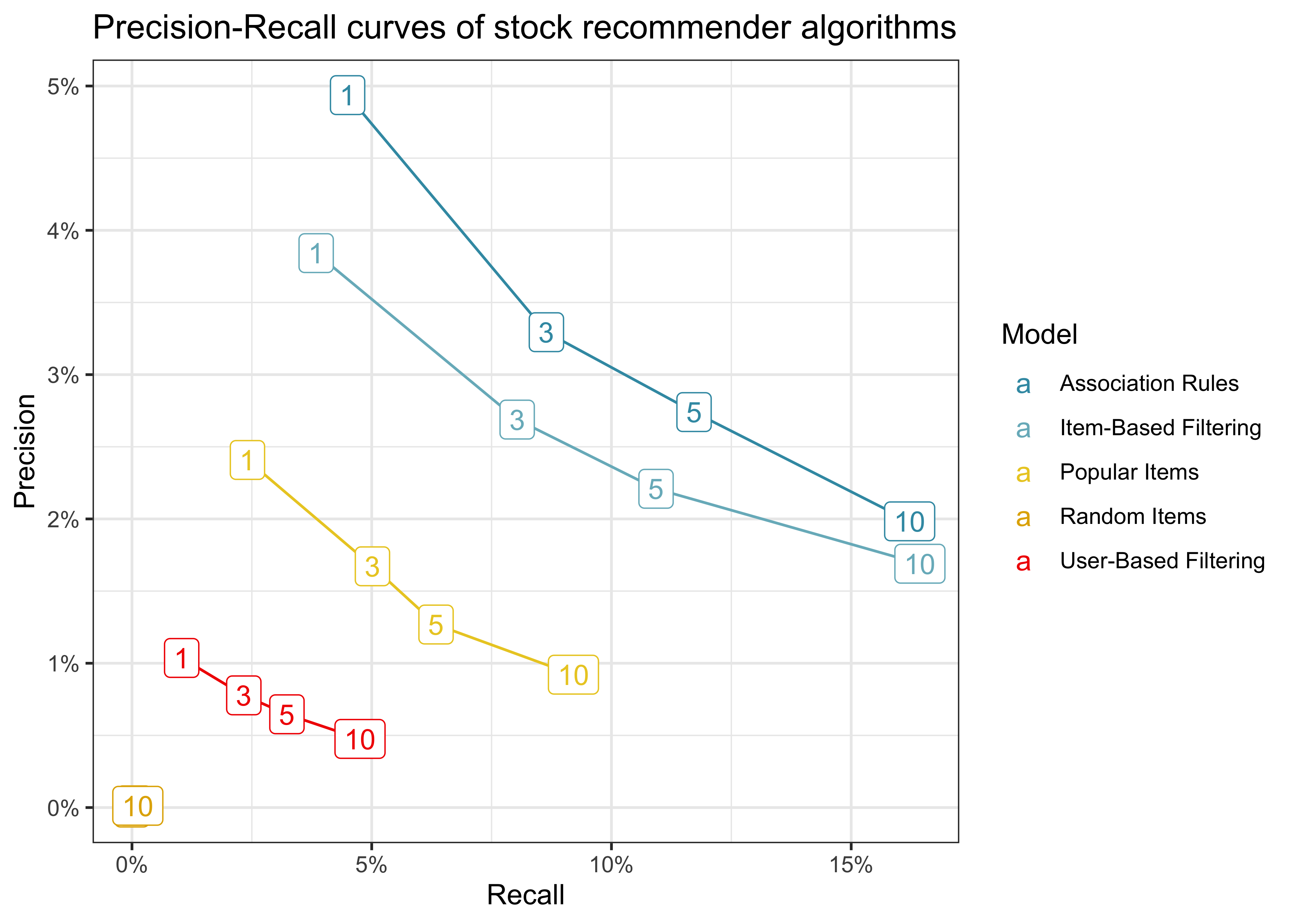

Title: Precision-Recall curves of stock recommender algorithms. The figure shows that the association rules mining algorithm achieves the highest precision for any level of recall.

Again, proposing random items exhibits the worst performance, as for any given level of recall, this approach has the lowest precision. Association rules are also the best algorithm with this visualization approach.

Create Predictions

The final step is to create stock recommendations for investors who already have portfolios. I pick the AR algorithm to create such recommendations because it excelled in the analyses above. Note that in the case of association rules, I also need to provide the support and confidence parameters.

recommender <- Recommender(binary_rating_matrix, method = "AR", param = list(supp = 0.01, conf = 0.1))

As an example, suppose you currently have a portfolio that consists of Nvidia (US67066G1040) and Apple (US0378331005). I have to transform this sample portfolio into a rating matrix with the same dimensions as the data we used as input for our training. The predict() function then delivers a prediction for the example portfolio.

sample_portfolio <- c("US67066G1040", "US0378331005")
sample_rating_matrix <- tibble(distinct(wikifolio_portfolios, stock)) |>
  mutate(in_portfolio = if_else(stock %in% sample_portfolio, 1, 0)) |>
  pivot_wider(names_from = stock,
              values_from = in_portfolio,
              values_fill = list(in_portfolio = 0)) |>
  as.matrix() |>
  as("binaryRatingMatrix")

prediction <- predict(recommender, sample_rating_matrix, n = 1)
as(prediction, "list")[[1]]

[1] "US5949181045"

So the AR algorithm recommends Microsoft (US5949181045) as a stock if you are already invested in Nvidia and Apple, which makes a lot of sense given the similarity in business model. Of course, this recommendation is not serious investment advice, but rather serves an illustrative purpose of how recommenderlab can be used to quickly prototype different collaborative filtering recommender algorithms.

References

Wickham, Hadley, Mara Averick, Jennifer Bryan, Winston Chang, Lucy D’Agostino McGowan, Romain François, Garrett Grolemund, et al. 2019. “Welcome to the Tidyverse.” Journal of Open Source Software 4 (43): 1686. https://doi.org/10.21105/joss.01686.

Wickham, Hadley, and Dana Seidel. 2022. scales: Scale functions for visualization. https://CRAN.R-project.org/package=scales.

Footnotes

Ricci, F, Rokach, L., Shapira, B. and Kantor, P. (2011). “Recommender Systems Handbook”. https://link.springer.com/book/10.1007/978-0-387-85820-3.↩︎
Hahsler, M. (2022). “recommenderlab: An R Framework for Developing and Testing Recommendation Algorithms”, R package version 1.0.3. https://CRAN.R-project.org/package=recommenderlab.↩︎
Breese, J.S., Heckerman, D. and Kadie, C. (1998). “Empirical Analysis of Predictive Algorithms for Collaborative Filtering”, Proceedings of the Fourteenth Conference on Uncertainty in Artificial Intelligence, Madison, 43-52. https://arxiv.org/pdf/1301.7363.pdf.↩︎