import pandas as pd
import numpy as np
import sqlite3
import statsmodels.formula.api as smf

from regtabletotext import prettify_result
from statsmodels.regression.rolling import RollingOLS
from plotnine import *
from mizani.breaks import date_breaks
from mizani.formatters import percent_format, date_format
from joblib import Parallel, delayed, cpu_count
from itertools import productBeta Estimation
Note
You are reading Tidy Finance with Python. You can find the equivalent chapter for the sibling Tidy Finance with R here.
In this chapter, we introduce an important concept in financial economics: The exposure of an individual stock to changes in the market portfolio. According to the Capital Asset Pricing Model (CAPM) of Sharpe (1964), Lintner (1965), and Mossin (1966), cross-sectional variation in expected asset returns should be a function of the covariance between the excess return of the asset and the excess return on the market portfolio. The regression coefficient of excess market returns on excess stock returns is usually called the market beta. We show an estimation procedure for the market betas. We do not go into details about the foundations of market beta but simply refer to any treatment of the CAPM for further information. Instead, we provide details about all the functions that we use to compute the results. In particular, we leverage useful computational concepts: Rolling-window estimation and parallelization.
We use the following Python packages throughout this chapter:
Compared to previous chapters, we introduce statsmodels (Seabold and Perktold 2010) for regression analysis and for sliding-window regressions and joblib (Team 2023) for parallelization.
Estimating Beta Using Monthly Returns
The estimation procedure is based on a rolling-window estimation, where we may use either monthly or daily returns and different window lengths. First, let us start with loading the monthly CRSP data from our SQLite database introduced in Accessing and Managing Financial Data and WRDS, CRSP, and Compustat.
tidy_finance = sqlite3.connect(database="data/tidy_finance_python.sqlite")

crsp_monthly = (pd.read_sql_query(
    sql="SELECT permno, date, industry, ret_excess FROM crsp_monthly",
    con=tidy_finance,
    parse_dates={"date"})
  .dropna()
)

factors_ff3_monthly = pd.read_sql_query(
  sql="SELECT date, mkt_excess FROM factors_ff3_monthly",
  con=tidy_finance,
  parse_dates={"date"}
)

crsp_monthly = (crsp_monthly
  .merge(factors_ff3_monthly, how="left", on="date")
)
To estimate the CAPM regression coefficients \[
r_{i, t} - r_{f, t} = \alpha_i + \beta_i(r_{m, t}-r_{f,t})+\varepsilon_{i, t},
\tag{1}\] we regress stock excess returns ret_excess on excess returns of the market portfolio mkt_excess.
Python provides a simple solution to estimate (linear) models with the function smf.ols(). The function requires a formula as input that is specified in a compact symbolic form. An expression of the form y ~ model is interpreted as a specification that the response y is modeled by a linear predictor specified symbolically by model. Such a model consists of a series of terms separated by + operators. In addition to standard linear models, smf.ols() provides a lot of flexibility. You should check out the documentation for more information. To start, we restrict the data only to the time series of observations in CRSP that correspond to Apple’s stock (i.e., to permno 14593 for Apple) and compute \(\hat\alpha_i\) as well as \(\hat\beta_i\).
model_beta = (smf.ols(
    formula="ret_excess ~ mkt_excess",
    data=crsp_monthly.query("permno == 14593"))
  .fit()
)
prettify_result(model_beta)
OLS Model:
ret_excess ~ mkt_excess
Coefficients:
Estimate Std. Error t-Statistic p-Value
Intercept 0.010 0.005 2.046 0.041
mkt_excess 1.384 0.109 12.696 0.000
Summary statistics:
- Number of observations: 516
- R-squared: 0.239, Adjusted R-squared: 0.237
- F-statistic: 161.191 on 1 and 514 DF, p-value: 0.000
smf.ols() returns an object of class RegressionModel, which contains all the information we usually care about with linear models. prettify_result() returns an overview of the estimated parameters. The output above indicates that Apple moves excessively with the market as the estimated \(\hat\beta_i\) is above one (\(\hat\beta_i \approx 1.4\)).
Rolling-Window Estimation
After we estimated the regression coefficients on an example, we scale the estimation of \(\beta_i\) to a whole different level and perform rolling-window estimations for the entire CRSP sample.
We take a total of five years of data (window_size) and require at least 48 months with return data to compute our betas (min_obs). Check out the Exercises if you want to compute beta for different time periods. We first identify firm identifiers (permno) for which CRSP contains sufficiently many records.
window_size = 60
min_obs = 48

valid_permnos = (crsp_monthly
  .dropna()
  .groupby("permno")["permno"]
  .count()
  .reset_index(name="counts")
  .query(f"counts > {window_size}+1")
)
Before we proceed with the estimation, one important issue is worth emphasizing: RollingOLS returns the estimated parameters of a linear regression by incorporating a window of the last window_size rows. Whenever monthly returns are implicitly missing (which means there is simply no entry recorded, e.g., because a company was delisted and only traded publicly again later), such a fixed window size may cause outdated observations to influence the estimation results. We thus recommend making such implicit missing rows explicit.
We hence collect information about the first and last listing date of each permno.
permno_information = (crsp_monthly
  .merge(valid_permnos, how="inner", on="permno")
  .groupby(["permno"])
  .aggregate(first_date=("date", "min"),
             last_date=("date", "max"))
  .reset_index()
)
To complete the missing observations in the CRSP sample, we obtain all possible permno-month combinations.
unique_permno = crsp_monthly["permno"].unique()
unique_month = factors_ff3_monthly["date"].unique()

all_combinations = pd.DataFrame(
  product(unique_permno, unique_month),
  columns=["permno", "date"]
)
Finally, we expand the CRSP sample and include a row (with missing excess returns) for each possible permno-date observation that falls within the start and end date where the respective permno has been publicly listed.
returns_monthly = (all_combinations
  .merge(crsp_monthly.get(["permno", "date", "ret_excess"]),
         how="left", on=["permno", "date"])
  .merge(permno_information, how="left", on="permno")
  .query("(date >= first_date) & (date <= last_date)")
  .drop(columns=["first_date", "last_date"])
  .merge(crsp_monthly.get(["permno", "date", "industry"]),
         how="left", on=["permno", "date"])
  .merge(factors_ff3_monthly, how="left", on="date")
)
The following function implements the CAPM regression for a dataframe (or a part thereof) containing at least min_obs observations to avoid huge fluctuations if the time series is too short. If the condition is violated (i.e., the time series is too short) the function returns a missing value.
def roll_capm_estimation(data, window_size, min_obs):
    """Calculate rolling CAPM estimation."""

    data = data.sort_values("date")

    result = (RollingOLS.from_formula(
      formula="ret_excess ~ mkt_excess",
      data=data,
      window=window_size,
      min_nobs=min_obs,
      missing="drop")
      .fit()
      .params.get("mkt_excess")
    )

    result.index = data.index

    return result
Before we approach the whole CRSP sample, let us focus on a couple of examples for well-known firms.
examples = pd.DataFrame({
  "permno": [14593, 10107, 93436, 17778],
  "company": ["Apple", "Microsoft", "Tesla", "Berkshire Hathaway"]
})
It is actually quite simple to perform the rolling-window estimation for an arbitrary number of stocks, which we visualize in the following code chunk and the resulting Figure 1.
beta_example = (returns_monthly
  .merge(examples, how="inner", on="permno")
  .groupby(["permno"])
  .apply(lambda x: x.assign(
    beta=roll_capm_estimation(x, window_size, min_obs))
  )
  .reset_index(drop=True)
  .dropna()
)
plot_beta = (
ggplot(
beta_example,
aes(x="date", y="beta", color="company", linetype="company")
)
+ geom_line()
+ labs(
x="", y="", color="", linetype="",
title="Monthly beta estimates for example stocks"
)
+ scale_x_datetime(breaks=date_breaks("5 year"), labels=date_format("%Y"))
)
plot_beta.show()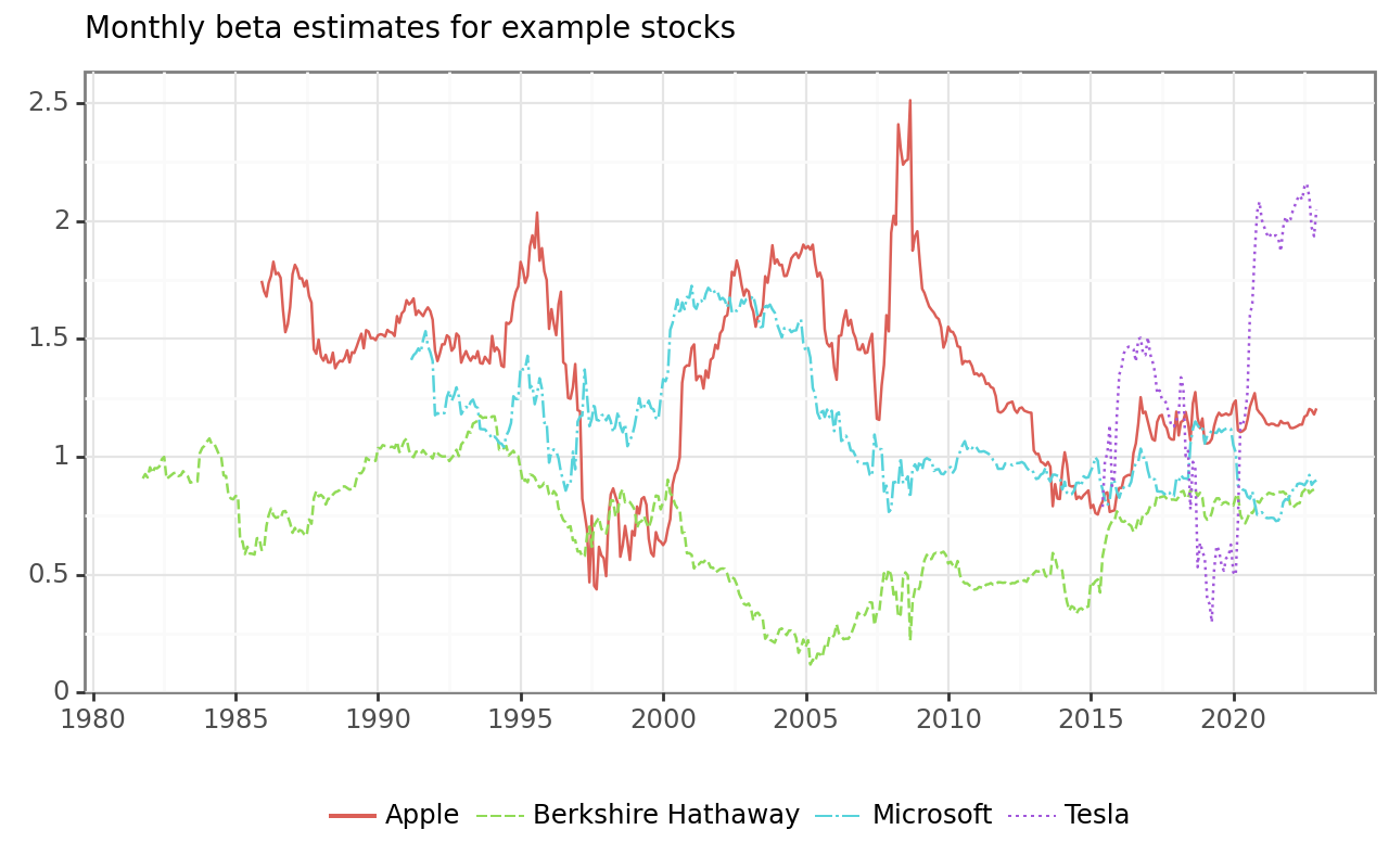
Parallelized Rolling-Window Estimation
Next, we perform the rolling window estimation for the entire cross-section of stocks in the CRSP sample. For that purpose, we can apply the code snippet from the example above to compute rolling window regression coefficients for all stocks. This is how to do it with the joblib package to use multiple cores. Note that we use cpu_count() to determine the number of cores available for parallelization but keep one core free for other tasks. Some machines might freeze if all cores are busy with Python jobs.
def roll_capm_estimation_for_joblib(permno, group):
    """Calculate rolling CAPM estimation using joblib."""

    group = group.sort_values(by="date")

    beta_values = (RollingOLS.from_formula(
        formula="ret_excess ~ mkt_excess",
        data=group,
        window=window_size,
        min_nobs=min_obs,
        missing="drop"
      )
      .fit()
      .params.get("mkt_excess")
    )

    result = pd.DataFrame(beta_values)
    result.columns = ["beta"]
    result["date"] = group["date"].values
    result["permno"] = permno

    return result

permno_groups = (returns_monthly
  .merge(valid_permnos, how="inner", on="permno")
  .groupby("permno", group_keys=False)
)

n_cores = cpu_count()-1

beta_monthly = (
  pd.concat(
    Parallel(n_jobs=n_cores)
    (delayed(roll_capm_estimation_for_joblib)(name, group)
    for name, group in permno_groups)
  )
  .dropna()
  .rename(columns={"beta": "beta_monthly"})
)
Estimating Beta Using Daily Returns
Before we provide some descriptive statistics of our beta estimates, we implement the estimation for the daily CRSP sample as well. Depending on the application, you might either use longer horizon beta estimates based on monthly data or shorter horizon estimates based on daily returns. As loading the full daily CRSP data requires relatively large amounts of memory, we split the beta estimation into smaller chunks. The logic follows the approach that we use to download the daily CRSP data (see WRDS, CRSP, and Compustat).
First, we load the daily Fama-French market excess returns and extract the vector of dates.
factors_ff3_daily = pd.read_sql_query(
  sql="SELECT date, mkt_excess FROM factors_ff3_daily",
  con=tidy_finance,
  parse_dates={"date"}
)

unique_date = factors_ff3_daily["date"].unique()
For the daily data, we consider around three months of data (i.e., 60 trading days), require at least 50 observations, and estimate betas in batches of 500.
window_size = 60
min_obs = 50

permnos = list(crsp_monthly["permno"].unique().astype(str))

batch_size = 500
batches = np.ceil(len(permnos)/batch_size).astype(int)
We then proceed to perform the same steps as with the monthly CRSP data, just in batches: Load in daily returns, transform implicit missing returns to explicit ones, keep only valid stocks with a minimum number of rows, and parallelize the beta estimation across stocks.
beta_daily = []

for j in range(1, batches+1):

    permno_batch = permnos[
      ((j-1)*batch_size):(min(j*batch_size, len(permnos)))
    ]

    permno_batch_formatted = (
      ", ".join(f"'{permno}'" for permno in permno_batch)
    )
    permno_string = f"({permno_batch_formatted})"

    crsp_daily_sub_query = (
      "SELECT permno, date, ret_excess "
        "FROM crsp_daily "
       f"WHERE permno IN {permno_string}"
    )

    crsp_daily_sub = pd.read_sql_query(
      sql=crsp_daily_sub_query,
      con=tidy_finance,
      dtype={"permno": int},
      parse_dates={"date"}
    )

    valid_permnos = (crsp_daily_sub
      .groupby("permno")["permno"]
      .count()
      .reset_index(name="counts")
      .query(f"counts > {window_size}+1")
      .drop(columns="counts")
    )

    permno_information = (crsp_daily_sub
      .merge(valid_permnos, how="inner", on="permno")
      .groupby(["permno"])
      .aggregate(first_date=("date", "min"),
                 last_date=("date", "max"),)
      .reset_index()
    )

    unique_permno = permno_information["permno"].unique()

    all_combinations = pd.DataFrame(
      product(unique_permno, unique_date),
      columns=["permno", "date"]
    )

    returns_daily = (crsp_daily_sub
      .merge(all_combinations, how="right", on=["permno", "date"])
      .merge(permno_information, how="left", on="permno")
      .query("(date >= first_date) & (date <= last_date)")
      .drop(columns=["first_date", "last_date"])
      .merge(factors_ff3_daily, how="left", on="date")
    )

    permno_groups = (returns_daily
      .groupby("permno", group_keys=False)
    )

    beta_daily_sub = (
      pd.concat(
        Parallel(n_jobs=n_cores)
        (delayed(roll_capm_estimation_for_joblib)(name, group)
        for name, group in permno_groups)
      )
      .dropna()
      .rename(columns={"beta": "beta_daily"})
    )

    beta_daily_sub = (beta_daily_sub
      .assign(
          month = lambda x:
            x["date"].dt.to_period("M").dt.to_timestamp()
        )
      .sort_values("date")
      .groupby(["permno", "month"])
      .last()
      .reset_index()
      .drop(columns="date")
      .rename(columns={"month": "date"})
    )

    beta_daily.append(beta_daily_sub)

    print(f"Batch {j} out of {batches} done ({(j/batches)*100:.2f}%)\n")

beta_daily = pd.concat(beta_daily)
Comparing Beta Estimates
What is a typical value for stock betas? To get some feeling, we illustrate the dispersion of the estimated \(\hat\beta_i\) across different industries and across time below. Figure 2 shows that typical business models across industries imply different exposure to the general market economy. However, there are barely any firms that exhibit a negative exposure to the market factor.
beta_industries = (beta_monthly
  .merge(crsp_monthly, how="inner", on=["permno", "date"])
  .dropna(subset="beta_monthly")
  .groupby(["industry","permno"])["beta_monthly"]
  .aggregate("mean")
  .reset_index()
)

industry_order = (beta_industries
  .groupby("industry")["beta_monthly"]
  .aggregate("median")
  .sort_values()
  .index.tolist()
)

plot_beta_industries = (
  ggplot(
    beta_industries,
    aes(x="industry", y="beta_monthly")
  )
  + geom_boxplot()
  + coord_flip()
  + labs(
      x="", y="",
      title="Firm-specific beta distributions by industry"
    )
  + scale_x_discrete(limits=industry_order)
)
plot_beta_industries.show()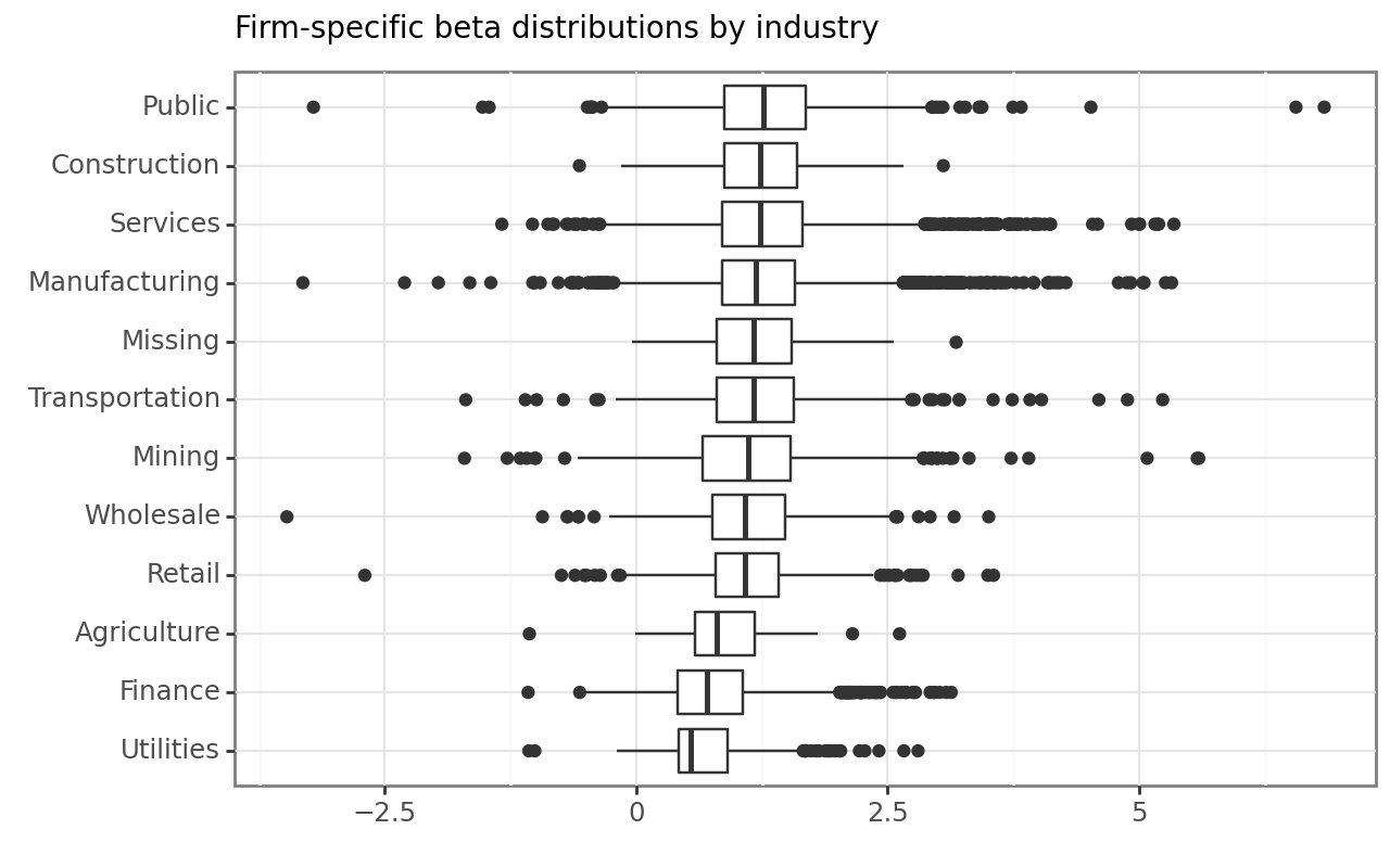
Next, we illustrate the time-variation in the cross-section of estimated betas. Figure 3 shows the monthly deciles of estimated betas (based on monthly data) and indicates an interesting pattern: First, betas seem to vary over time in the sense that during some periods, there is a clear trend across all deciles. Second, the sample exhibits periods where the dispersion across stocks increases in the sense that the lower decile decreases and the upper decile increases, which indicates that for some stocks, the correlation with the market increases, while for others it decreases. Note also here: stocks with negative betas are a rare exception.
beta_quantiles = (beta_monthly
  .groupby("date")["beta_monthly"]
  .quantile(q=np.arange(0.1, 1.0, 0.1))
  .reset_index()
  .rename(columns={"level_1": "quantile"})
  .assign(quantile=lambda x: (x["quantile"]*100).astype(int))
  .dropna()
)

linetypes = ["-", "--", "-.", ":"]
n_quantiles = beta_quantiles["quantile"].nunique()

plot_beta_quantiles = (
  ggplot(
    beta_quantiles,
    aes(x="date", y="beta_monthly", color="factor(quantile)", linetype="factor(quantile)")
  )
  + geom_line()
  + labs(
      x="", y="", color="", linetype="",
      title="Monthly deciles of estimated betas"
    )
  + scale_x_datetime(breaks=date_breaks("5 year"), labels=date_format("%Y"))
  + scale_linetype_manual(
      values=[linetypes[l % len(linetypes)] for l in range(n_quantiles)]
    )
)
plot_beta_quantiles.show()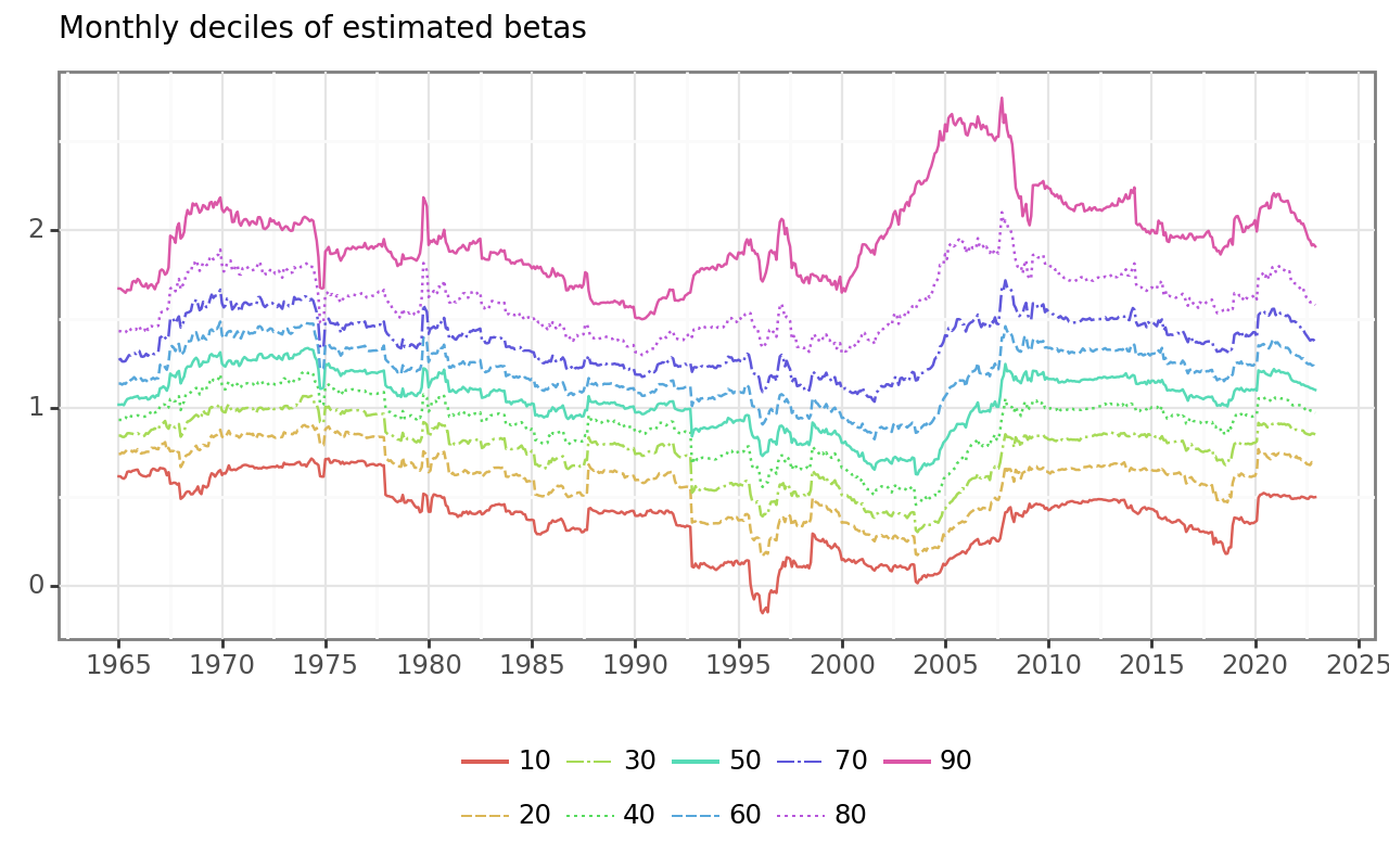
To compare the difference between daily and monthly data, we combine beta estimates to a single table. Then, we use the table to plot a comparison of beta estimates for our example stocks in Figure 4.
beta = (beta_monthly
  .get(["permno", "date", "beta_monthly"])
  .merge(beta_daily.get(["permno", "date", "beta_daily"]),
         how="outer", on=["permno", "date"])
)

beta_comparison = (beta
  .merge(examples, on="permno")
  .melt(id_vars=["permno", "date", "company"], var_name="name",
        value_vars=["beta_monthly", "beta_daily"], value_name="value")
  .dropna()
)

plot_beta_comparison = (
  ggplot(
    beta_comparison,
    aes(x="date", y="value", color="name")
  )
  + geom_line()
  + facet_wrap("~company", ncol=1)
  + labs(
      x="", y="", color="",
      title="Comparison of beta estimates using monthly and daily data"
    )
  + scale_x_datetime(breaks=date_breaks("10 years"), labels=date_format("%Y"))
  + theme(figure_size=(6.4, 6.4))
)
plot_beta_comparison.show()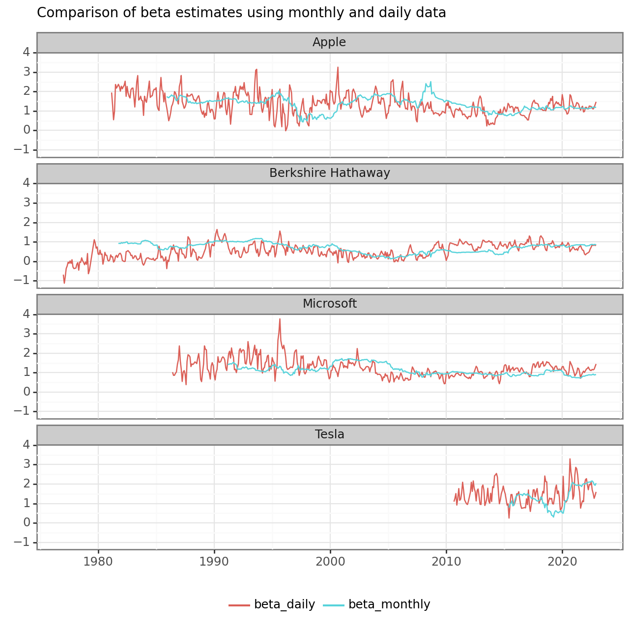
The estimates in Figure 4 look as expected. As you can see, the beta estimates really depend on the estimation window and data frequency. Nevertheless, one can observe a clear connection between daily and monthly betas in this example, in magnitude and the dynamics over time.
Finally, we write the estimates to our database so that we can use them in later chapters.
(beta.to_sql(
  name="beta",
  con=tidy_finance,
  if_exists="replace",
  index=False
  )
)
Whenever you perform some kind of estimation, it also makes sense to do rough plausibility tests. A possible check is to plot the share of stocks with beta estimates over time. This descriptive analysis helps us discover potential errors in our data preparation or the estimation procedure. For instance, suppose there was a gap in our output without any betas. In this case, we would have to go back and check all previous steps to find out what went wrong. Figure 5 does not indicate any troubles, so let us move on to the next check.
beta_long = (crsp_monthly
  .merge(beta, how="left", on=["permno", "date"])
  .melt(id_vars=["permno", "date"], var_name="name",
        value_vars=["beta_monthly", "beta_daily"], value_name="value")
)

beta_shares = (beta_long
  .groupby(["date", "name"])
  .aggregate(share=("value", lambda x: sum(~x.isna())/len(x)))
  .reset_index()
)

plot_beta_long = (
  ggplot(
    beta_shares,
    aes(x="date", y="share", color="name", linetype="name")
  )
  + geom_line()
  + labs(
      x="", y="", color="", linetype="",
      title="End-of-month share of securities with beta estimates"
    )
  + scale_y_continuous(labels=percent_format())
  + scale_x_datetime(breaks=date_breaks("10 year"), labels=date_format("%Y"))
)
plot_beta_long.show()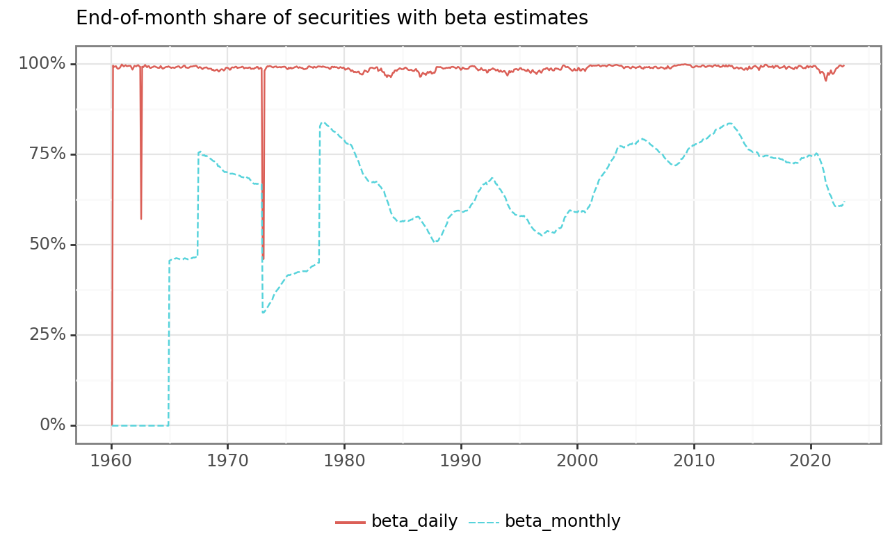
We also encourage everyone to always look at the distributional summary statistics of variables. You can easily spot outliers or weird distributions when looking at such tables.
beta_long.groupby("name")["value"].describe().round(2)| count | mean | std | min | 25% | 50% | 75% | max | |
|---|---|---|---|---|---|---|---|---|
| name | ||||||||
| beta_daily | 3326419.0 | 0.76 | 0.94 | -44.85 | 0.21 | 0.69 | 1.24 | 61.64 |
| beta_monthly | 2103719.0 | 1.10 | 0.70 | -8.96 | 0.64 | 1.03 | 1.47 | 10.35 |
The summary statistics also look plausible for the two estimation procedures.
Finally, since we have two different estimators for the same theoretical object, we expect the estimators to be at least positively correlated (although not perfectly as the estimators are based on different sample periods and frequencies).
beta.get(["beta_monthly", "beta_daily"]).corr().round(2)| beta_monthly | beta_daily | |
|---|---|---|
| beta_monthly | 1.00 | 0.32 |
| beta_daily | 0.32 | 1.00 |
Indeed, we find a positive correlation between our beta estimates. In the subsequent chapters, we mainly use the estimates based on monthly data, as most readers should be able to replicate them and should not encounter potential memory limitations that might arise with the daily data.
Key Takeaways
- CAPM betas can be estimated using rolling-window estimation via the
statsmodelspackage and processed in parallel viajoblib. - Both monthly and daily return data can be used to estimate betas with different frequencies and window lengths, depending on the application.
- Summary statistics, visualization, and plausibility checks help to validate beta estimates across time and industries.
- The
tidyfinancePython package provides a user-friendlyestimate_betas()function that simplifies the full beta estimation pipeline.
Exercises
- Compute beta estimates based on monthly data using one, three, and five years of data and impose a minimum number of observations of 10, 28, and 48 months with return data, respectively. How strongly correlated are the estimated betas?
- Compute beta estimates based on monthly data using five years of data and impose different numbers of minimum observations. How does the share of
permno-dateobservations with successful beta estimates vary across the different requirements? Do you find a high correlation across the estimated betas? - Instead of using
joblib, perform the beta estimation in a loop (using either monthly or daily data) for a subset of 100 permnos of your choice. Verify that you get the same results as with the parallelized code from above. - Filter out the stocks with negative betas. Do these stocks frequently exhibit negative betas, or do they resemble estimation errors?
- Compute beta estimates for multi-factor models such as the Fama-French three-factor model. For that purpose, you extend your regression to \[ r_{i, t} - r_{f, t} = \alpha_i + \sum\limits_{j=1}^k\beta_{i,k}(r_{j, t}-r_{f,t})+\varepsilon_{i, t} \tag{2}\] where \(r_{i, t}\) are the \(k\) factor returns. Thus, you estimate four parameters (\(\alpha_i\) and the slope coefficients). Provide some summary statistics of the cross-section of firms and their exposure to the different factors.
References
Lintner, John. 1965. “Security prices, risk, and maximal gains from diversification.” The Journal of Finance 20 (4): 587–615. https://doi.org/10.1111/j.1540-6261.1965.tb02930.x.
Mossin, Jan. 1966. “Equilibrium in a capital asset market.” Econometrica 34 (4): 768–83. https://doi.org/10.2307/1910098.
Seabold, Skipper, and Josef Perktold. 2010. “Statsmodels: Econometric and Statistical Modeling with Python.” In 9th Python in Science Conference.
Sharpe, William F. 1964. “Capital asset prices: A theory of market equilibrium under conditions of risk .” The Journal of Finance 19 (3): 425–42. https://doi.org/10.1111/j.1540-6261.1964.tb02865.x.
Team, Joblib Development. 2023. “Joblib: Running Python Functions as Pipeline Jobs.” https://joblib.readthedocs.io/.