import pandas as pd
import numpy as np
import sqlite3

from plotnine import *
from mizani.formatters import percent_format, date_format
from mizani.breaks import date_breaks
from itertools import product
from sklearn.model_selection import (
  train_test_split, GridSearchCV, TimeSeriesSplit, cross_val_score
)
from sklearn.compose import ColumnTransformer
from sklearn.preprocessing import StandardScaler
from sklearn.pipeline import Pipeline
from sklearn.linear_model import ElasticNet, Lasso, RidgeFactor Selection via Machine Learning
Note
You are reading Tidy Finance with Python. You can find the equivalent chapter for the sibling Tidy Finance with R here.
The aim of this chapter is twofold. From a data science perspective, we introduce scikit-learn, a collection of packages for modeling and machine learning (ML). scikit-learn comes with a handy workflow for all sorts of typical prediction tasks. From a finance perspective, we address the notion of factor zoo (Cochrane 2011) using ML methods. We introduce Lasso, Ridge, and Elastic Net regression as a special case of penalized regression models. Then, we explain the concept of cross-validation for model tuning with Elastic Net regularization as a popular example. We implement and showcase the entire cycle from model specification, training, and forecast evaluation within the scikit-learn universe. While the tools can generally be applied to an abundance of interesting asset pricing problems, we apply penalized regressions for identifying macroeconomic variables and asset pricing factors that help explain a cross-section of industry portfolios.
In previous chapters, we illustrate that stock characteristics such as size provide valuable pricing information in addition to the market beta. Such findings question the usefulness of the Capital Asset Pricing Model. In fact, during the last decades, financial economists discovered a plethora of additional factors which may be correlated with the marginal utility of consumption (and would thus deserve a prominent role in pricing applications). The search for factors that explain the cross-section of expected stock returns has produced hundreds of potential candidates, as noted more recently by Harvey, Liu, and Zhu (2016), Harvey (2017), Mclean and Pontiff (2016), and Hou, Xue, and Zhang (2020). Therefore, given the multitude of proposed risk factors, the challenge these days rather is: do we believe in the relevance of hundreds of risk factors? During recent years, promising methods from the field of ML got applied to common finance applications. We refer to Mullainathan and Spiess (2017) for a treatment of ML from the perspective of an econometrician, Nagel (2021) for an excellent review of ML practices in asset pricing, Easley et al. (2020) for ML applications in (high-frequency) market microstructure, and Dixon, Halperin, and Bilokon (2020) for a detailed treatment of all methodological aspects.
Brief Theoretical Background
This is a book about doing empirical work in a tidy manner, and we refer to any of the many excellent textbook treatments of ML methods and especially penalized regressions for some deeper discussion. Excellent material is provided, for instance, by Hastie, Tibshirani, and Friedman (2009), Gareth et al. (2013), and De Prado (2018). Instead, we briefly summarize the idea of Lasso and Ridge regressions as well as the more general Elastic Net. Then, we turn to the fascinating question on how to implement, tune, and use such models with the scikit-learn package.
To set the stage, we start with the definition of a linear model: Suppose we have data \((y_t, x_t), t = 1,\ldots, T\), where \(x_t\) is a \((K \times 1)\) vector of regressors and \(y_t\) is the response for observation \(t\). The linear model takes the form \(y_t = \beta' x_t + \varepsilon_t\) with some error term \(\varepsilon_t\) and has been studied in abundance. For \(K\leq T\), the well-known ordinary-least square (OLS) estimator for the \((K \times 1)\) vector \(\beta\) minimizes the sum of squared residuals and is then \[\hat{\beta}^\text{ols} = \left(\sum\limits_{t=1}^T x_t'x_t\right)^{-1} \sum\limits_{t=1}^T x_t'y_t. \tag{1}\]
While we are often interested in the estimated coefficient vector \(\hat\beta^\text{ols}\), ML is about the predictive performance most of the time. For a new observation \(\tilde{x}_t\), the linear model generates predictions such that \[\hat y_t = E\left(y|x_t = \tilde x_t\right) = \hat\beta^\text{ols}{}' \tilde x_t. \tag{2}\] Is this the best we can do? Not necessarily: instead of minimizing the sum of squared residuals, penalized linear models can improve predictive performance by choosing other estimators \(\hat{\beta}\) with lower variance than the estimator \(\hat\beta^\text{ols}\). At the same time, it seems appealing to restrict the set of regressors to a few meaningful ones, if possible. In other words, if \(K\) is large (such as for the number of proposed factors in the asset pricing literature), it may be a desirable feature to select reasonable factors and set \(\hat\beta^{\text{ols}}_k = 0\) for some redundant factors.
It should be clear that the promised benefits of penalized regressions, i.e., reducing the mean squared error (MSE), come at a cost. In most cases, reducing the variance of the estimator introduces a bias such that \(E\left(\hat\beta\right) \neq \beta\). What is the effect of such a bias-variance trade-off? To understand the implications, assume the following data-generating process for \(y\): \[y = f(x) + \varepsilon, \quad \varepsilon \sim (0, \sigma_\varepsilon^2) \tag{3}\] We want to recover \(f(x)\), which denotes some unknown functional which maps the relationship between \(x\) and \(y\). While the properties of \(\hat\beta^\text{ols}\) as an unbiased estimator may be desirable under some circumstances, they are certainly not if we consider predictive accuracy. Alternative predictors \(\hat{f}(x)\) could be more desirable: For instance, the MSE depends on our model choice as follows: \[\begin{aligned} MSE &=E\left(\left(y-\hat{f}(x)\right)^2\right)=E\left(\left(f(x)+\epsilon-\hat{f}(x)\right)^2\right)\\ &= \underbrace{E\left(\left(f(x)-\hat{f}(x)\right)^2\right)}_{\text{total quadratic error}}+\underbrace{E\left(\epsilon^2\right)}_{\text{irreducible error}} \\ &= E\left(\hat{f}(x)^2\right)+E\left(f(x)^2\right)-2E\left(f(x)\hat{f}(x)\right)+\sigma_\varepsilon^2\\ &=E\left(\hat{f}(x)^2\right)+f(x)^2-2f(x)E\left(\hat{f}(x)\right)+\sigma_\varepsilon^2\\ &=\underbrace{\text{Var}\left(\hat{f}(x)\right)}_{\text{variance of model}}+ \underbrace{\left(E(f(x)-\hat{f}(x))\right)^2}_{\text{squared bias}} +\sigma_\varepsilon^2. \end{aligned} \tag{4}\] While no model can reduce \(\sigma_\varepsilon^2\), a biased estimator with small variance may have a lower MSE than an unbiased estimator.
Ridge regression
One biased estimator is known as Ridge regression. Hoerl and Kennard (1970) propose to minimize the sum of squared errors while simultaneously imposing a penalty on the \(L_2\) norm of the parameters \(\hat\beta\). Formally, this means that for a penalty factor \(\lambda\geq 0\), the minimization problem takes the form \(\min_\beta \left(y - X\beta\right)'\left(y - X\beta\right)\text{ s.t. } \beta'\beta \leq c\). Here \(c\geq 0\) is a constant that depends on the choice of \(\lambda\). The larger \(\lambda\), the smaller \(c\) (technically speaking, there is a one-to-one relationship between \(\lambda\), which corresponds to the Lagrangian of the minimization problem above and \(c\)). Here, \(X = \left(x_1 \ldots x_T\right)'\) and \(y = \left(y_1, \ldots, y_T\right)'\). A closed-form solution for the resulting regression coefficient vector \(\beta^\text{ridge}\) exists: \[\hat{\beta}^\text{ridge} = \left(X'X + \lambda I\right)^{-1}X'y, \tag{5}\] where \(I\) is the identity matrix of dimension \(K\). A couple of observations are worth noting: \(\hat\beta^\text{ridge} = \hat\beta^\text{ols}\) for \(\lambda = 0\) and \(\hat\beta^\text{ridge} \rightarrow 0\) for \(\lambda\rightarrow \infty\). Also for \(\lambda > 0\), \(\left(X'X + \lambda I\right)\) is non-singular even if \(X'X\) is which means that \(\hat\beta^\text{ridge}\) exists even if \(\hat\beta\) is not defined. However, note also that the Ridge estimator requires careful choice of the hyperparameter \(\lambda\) which controls the amount of regularization: a larger value of \(\lambda\) implies shrinkage of the regression coefficient toward 0; a smaller value of \(\lambda\) reduces the bias of the resulting estimator.
Note that \(X\) usually contains an intercept column with ones. As a general rule, the associated intercept coefficient is not penalized. In practice, this often implies that \(y\) is simply demeaned before computing \(\hat\beta^\text{ridge}\).
What about the statistical properties of the Ridge estimator? First, the bad news is that \(\hat\beta^\text{ridge}\) is a biased estimator of \(\beta\). However, the good news is that (under homoscedastic error terms) the variance of the Ridge estimator is guaranteed to be smaller than the variance of the OLS estimator. We encourage you to verify these two statements in the Exercises. As a result, we face a trade-off: The Ridge regression sacrifices some unbiasedness to achieve a smaller variance than the OLS estimator.
Lasso
An alternative to Ridge regression is the Lasso (least absolute shrinkage and selection operator). Similar to Ridge regression, the Lasso (Tibshirani 1996) is a penalized and biased estimator. The main difference to Ridge regression is that Lasso does not only shrink coefficients but effectively selects variables by setting coefficients for irrelevant variables to zero. Lasso implements a \(L_1\) penalization on the parameters such that: \[\hat\beta^\text{Lasso} = \arg\min_\beta \left(Y - X\beta\right)'\left(Y - X\beta\right)\text{ s.t. } \sum\limits_{k=1}^K|\beta_k| < c(\lambda). \tag{6}\] There is no closed-form solution for \(\hat\beta^\text{Lasso}\) in the above maximization problem, but efficient algorithms exist (e.g., the glmnet package for R and Python). Like for Ridge regression, the hyperparameter \(\lambda\) has to be specified beforehand.
The corresponding Lagrangian reads as follows \[\begin{aligned}\hat\beta_\lambda^\text{Lasso} = \arg\min_\beta \left(Y - X\beta\right)'\left(Y - X\beta\right) + \lambda\sum\limits_{k=1}^K|\beta_k|.\end{aligned} \tag{7}\]
Elastic Net
The Elastic Net (Zou and Hastie 2005) combines \(L_1\) with \(L_2\) penalization and encourages a grouping effect, where strongly correlated predictors tend to be in or out of the model together. In terms of the Lagrangian, this more general framework considers the following optimization problem: \[\hat\beta^\text{EN} = \arg\min_\beta \left(Y - X\beta\right)'\left(Y - X\beta\right) + \lambda(1-\rho)\sum\limits_{k=1}^K|\beta_k| +\frac{1}{2}\lambda\rho\sum\limits_{k=1}^K\beta_k^2 \tag{8}\] Now, we have to choose two hyperparameters: the shrinkage factor \(\lambda\) and the weighting parameter \(\rho\). The Elastic Net resembles Lasso for \(\rho = 0\) and Ridge regression for \(\rho = 1\). While the glmnet package provides efficient algorithms to compute the coefficients of penalized regressions, it is a good exercise to implement Ridge and Lasso estimation on your own before you use the scikit-learn back-end.
Python Packages
To get started, we load the required packages and data. The main focus is on the workflow behind the scikit-learn (Pedregosa et al. 2011) package collection.
Data Preparation
In this analysis, we use four different data sources that we load from our SQLite database introduced in Accessing and Managing Financial Data. We start with two different sets of factor portfolio returns which have been suggested as representing practical risk factor exposure and thus should be relevant when it comes to asset pricing applications.
- The standard workhorse: monthly Fama-French 3 factor returns (market, small-minus-big, and high-minus-low book-to-market valuation sorts) defined in Fama and French (1992) and Fama and French (1993).
- Monthly q-factor returns from Hou, Xue, and Zhang (2014). The factors contain the size factor, the investment factor, the return-on-equity factor, and the expected growth factor.
Next, we include macroeconomic predictors which may predict the general stock market economy. Macroeconomic variables effectively serve as conditioning information such that their inclusion hints at the relevance of conditional models instead of unconditional asset pricing. We refer the interested reader to Cochrane (2009) on the role of conditioning information.
- Our set of macroeconomic predictors comes from Welch and Goyal (2008). The data has been updated by the authors until 2021 and contains monthly variables that have been suggested as good predictors for the equity premium. Some of the variables are the dividend price ratio, earnings price ratio, stock variance, net equity expansion, treasury bill rate, and inflation.
Finally, we need a set of test assets. The aim is to understand which of the plenty factors and macroeconomic variable combinations prove helpful in explaining our test assets’ cross-section of returns. In line with many existing papers, we use monthly portfolio returns from ten different industries according to the definition from Kenneth French’s homepage as test assets.
tidy_finance = sqlite3.connect(database="data/tidy_finance_python.sqlite")

factors_ff3_monthly = (pd.read_sql_query(
     sql="SELECT * FROM factors_ff3_monthly",
     con=tidy_finance,
     parse_dates={"date"})
  .add_prefix("factor_ff_")
)

factors_q_monthly = (pd.read_sql_query(
    sql="SELECT * FROM factors_q_monthly",
    con=tidy_finance,
    parse_dates={"date"})
  .add_prefix("factor_q_")
)

macro_predictors = (pd.read_sql_query(
    sql="SELECT * FROM macro_predictors",
    con=tidy_finance,
    parse_dates={"date"})
 .add_prefix("macro_")
)

industries_ff_monthly = (pd.read_sql_query(
    sql="SELECT * FROM industries_ff_monthly",
    con=tidy_finance,
    parse_dates={"date"})
  .melt(id_vars="date", var_name="industry", value_name="ret")
)
We combine all the monthly observations into one dataframe.
data = (industries_ff_monthly
  .merge(factors_ff3_monthly,
         how="left", left_on="date", right_on="factor_ff_date")
  .merge(factors_q_monthly,
         how="left", left_on="date", right_on="factor_q_date")
  .merge(macro_predictors,
         how="left", left_on="date", right_on="macro_date")
  .assign(ret_excess=lambda x: x["ret"] - x["factor_ff_rf"])
  .drop(columns=["ret", "factor_ff_date", "factor_q_date", "macro_date"])
  .dropna()
)
Our data contains 23 columns of regressors with the 13 macro-variables and 9 factor returns for each month. Figure 1 provides summary statistics for the 10 monthly industry excess returns in percent. One can see that the dispersion in the excess returns varies widely across industries.
data_figure = (
  ggplot(
    data,
    aes(x="industry", y="ret_excess")
  )
  + geom_boxplot()
  + coord_flip()
  + labs(x="", y="", title="Excess return distributions by industry in percent")
  + scale_y_continuous(labels=percent_format())
)
data_figure.show()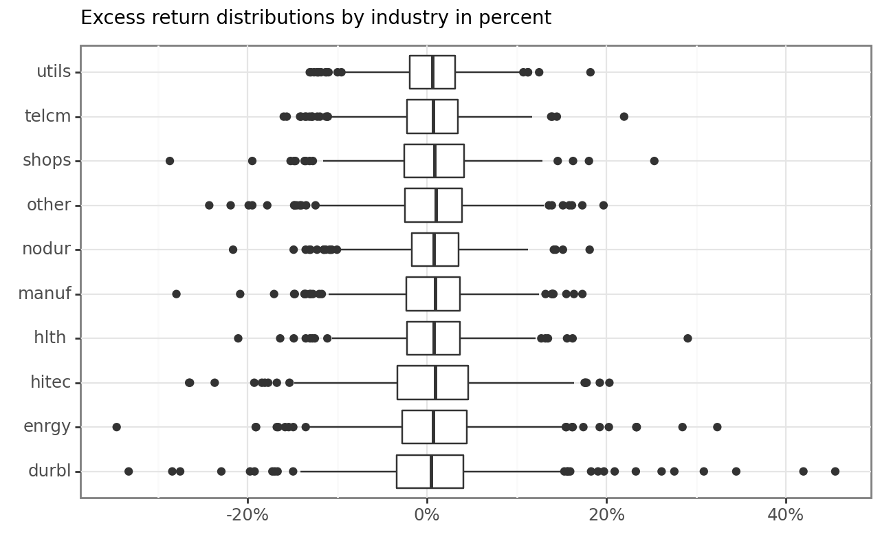
Machine Learning Workflow
To illustrate penalized linear regressions, we employ the scikit-learn collection of packages for modeling and ML. Using the ideas of Ridge and Lasso regressions, the following example guides you through (i) pre-processing the data (data split and variable mutation), (ii) building models, (iii) fitting models, and (iv) tuning models to create the “best” possible predictions.
Pre-process data
We want to explain excess returns with all available predictors. The regression equation thus takes the form \[r_{t} = \alpha_0 + \left(\tilde f_t \otimes \tilde z_t\right)B + \varepsilon_t \tag{9}\] where \(r_t\) is the vector of industry excess returns at time \(t\), \(\otimes\) denotes the Kronecker product and \(\tilde f_t\) and \(\tilde z_t\) are the (standardized) vectors of factor portfolio returns and macroeconomic variables.
We hence perform the following pre-processing steps:
- We exclude the column month from the analysis
- We include all interaction terms between factors and macroeconomic predictors
- We demean and scale each regressor such that the standard deviation is one
Scaling is often necessary in machine learning applications, especially when combining variables of different magnitudes or units, or when using algorithms sensitive to feature scales (e.g., gradient descent-based algorithms). We use ColumnTransformer() to scale all regressors using StandardScaler(). The remainder="drop" ensures that only the specified columns are retained in the output, and others are dropped. The option verbose_feature_names_out=False ensures that the output feature names remain unchanged. Also note that we use the zip() function to pair each element from column_names with its corresponding list of values from new_column_values, creating tuples, and then convert these tuples into a dictionary using dict() from which we create a dataframe.
macro_variables = data.filter(like="macro").columns
factor_variables = data.filter(like="factor").columns

column_combinations = list(product(macro_variables, factor_variables))

new_column_values = []
for macro_column, factor_column in column_combinations:
    new_column_values.append(data[macro_column] * data[factor_column])

column_names = [" x ".join(t) for t in column_combinations]
new_columns = pd.DataFrame(dict(zip(column_names, new_column_values)))

data = pd.concat([data, new_columns], axis=1)

preprocessor = ColumnTransformer(
  transformers=[
    ("scale", StandardScaler(),
    [col for col in data.columns
      if col not in ["ret_excess", "date", "industry"]])
  ],
  remainder="drop",
  verbose_feature_names_out=False
)
Build a model
Next, we can build an actual model based on our pre-processed data. In line with the definition above, we estimate regression coefficients of a Lasso regression such that we get
\[\begin{aligned}\hat\beta_\lambda^\text{Lasso} = \arg\min_\beta \left(Y - X\beta\right)'\left(Y - X\beta\right) + \lambda\sum\limits_{k=1}^K|\beta_k|.\end{aligned} \tag{10}\] In the application at hand, \(X\) contains 117 columns with all possible interactions between factor returns and macroeconomic variables. We want to emphasize that the workflow for any model is very similar, irrespective of the specific model. As you will see further below, it is straightforward to fit Ridge regression coefficients and, later, Neural networks or Random forests with similar code. For now, we start with the linear regression model with an arbitrarily chosen value for the penalty factor \(\lambda\) (denoted as alpha=0.007 in the code below). In the setup below, l1_ratio denotes the value of \(1-\rho\), hence setting l1_ratio=1 implies the Lasso.
lm_model = ElasticNet(
  alpha=0.007,
  l1_ratio=1,
  max_iter=5000,
  fit_intercept=False
)

lm_pipeline = Pipeline([
  ("preprocessor", preprocessor),
  ("regressor", lm_model)
])
That’s it - we are done! The object lm_model_pipeline contains the definition of our model with all required information, in particular the pre-processing steps and the regression model.
Fit a model
With the pipeline from above, we are ready to fit it to the data. Typically, we use training data to fit the model. The training data is pre-processed according to our recipe steps, and the Lasso regression coefficients are computed. For illustrative purposes, we focus on the manufacturing industry for now.
data_manufacturing = data.query("industry == 'manuf'")
training_date = "2011-12-01"

data_manufacturing_training = (data_manufacturing
  .query(f"date<'{training_date}'")
)

lm_fit = lm_pipeline.fit(
  data_manufacturing_training,
  data_manufacturing_training.get("ret_excess")
)
First, we focus on the in-sample predicted values \(\hat{y}_t = x_t\hat\beta^\text{Lasso}.\) Figure 2 illustrates the projections for the entire time series of the manufacturing industry portfolio returns.
predicted_values = (pd.DataFrame({
    "Fitted value": lm_fit.predict(data_manufacturing),
    "Realization": data_manufacturing.get("ret_excess")
  })
  .assign(date = data_manufacturing["date"])
  .melt(id_vars="date", var_name="Variable", value_name="return")
)

predicted_values_figure = (
  ggplot(
    predicted_values,
    aes(x="date", y="return", color="Variable", linetype="Variable")
  )
  + annotate(
    "rect",
    xmin=data_manufacturing_training["date"].max(),
    xmax=data_manufacturing["date"].max(),
    ymin=-np.inf, ymax=np.inf,
    alpha=0.25, fill="#808080"
  )
  + geom_line()
  + labs(
      x="", y="", color="", linetype="",
      title="Monthly realized and fitted manufacturing risk premia"
    )
  + scale_x_datetime(breaks=date_breaks("5 years"), labels=date_format("%Y"))
  + scale_y_continuous(labels=percent_format())
)
predicted_values_figure.show()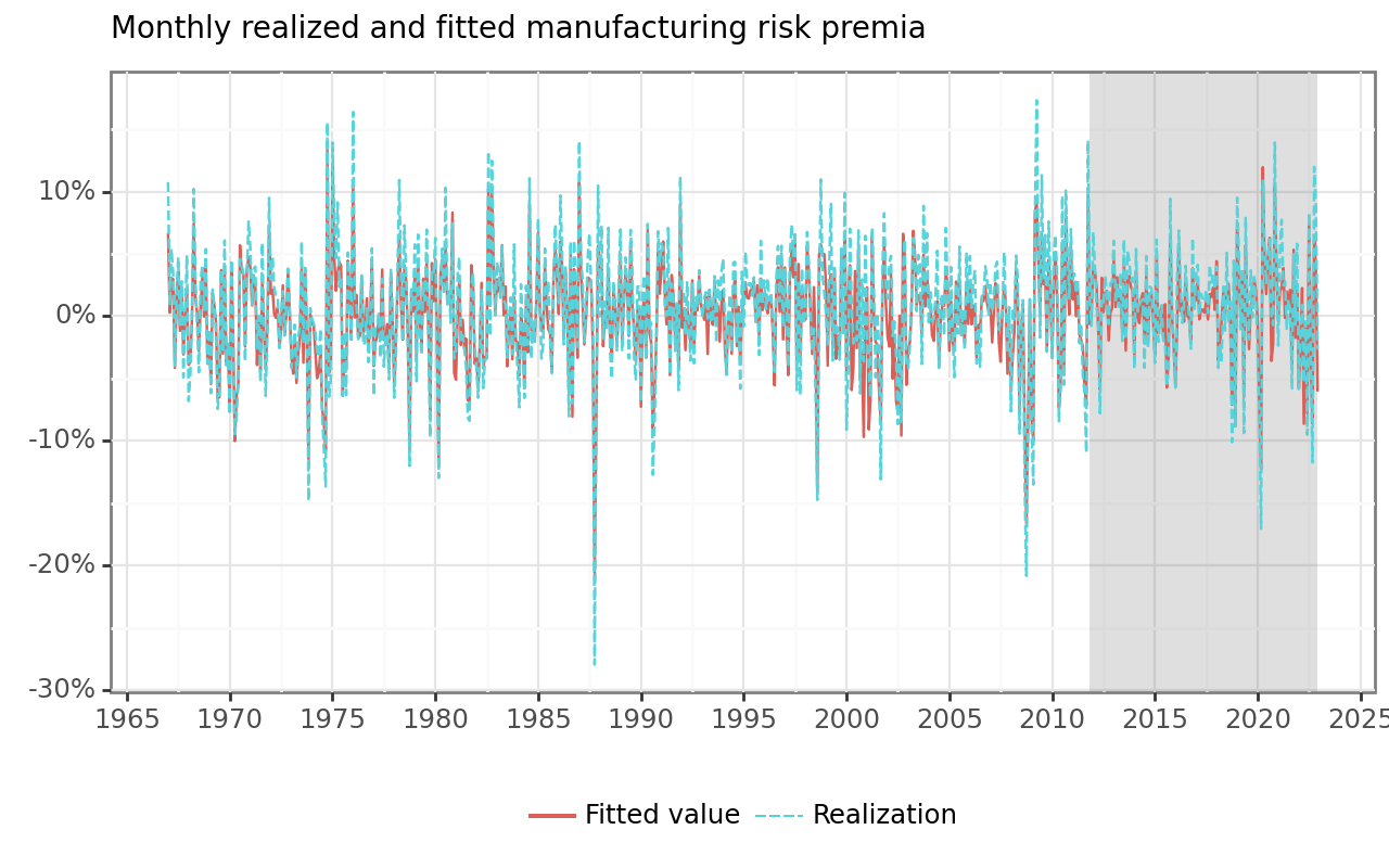
What do the estimated coefficients look like? To analyze these values, it is worth computing the coefficients \(\hat\beta^\text{Lasso}\) directly. The code below estimates the coefficients for the Lasso and Ridge regression for the processed training data sample for a grid of different \(\lambda\)’s.
x = preprocessor.fit_transform(data_manufacturing)
y = data_manufacturing["ret_excess"]

alphas = np.logspace(-5, 5, 100)

coefficients_lasso = []
for a in alphas:
    lasso = Lasso(alpha=a, fit_intercept=False)
    coefficients_lasso.append(lasso.fit(x, y).coef_)

coefficients_lasso = (pd.DataFrame(coefficients_lasso)
  .assign(alpha=alphas, model="Lasso")
  .melt(id_vars=["alpha", "model"])
)

coefficients_ridge = []
for a in alphas:
    ridge = Ridge(alpha=a, fit_intercept=False)
    coefficients_ridge.append(ridge.fit(x, y).coef_)

coefficients_ridge = (pd.DataFrame(coefficients_ridge)
  .assign(alpha=alphas, model="Ridge")
  .melt(id_vars=["alpha", "model"])
)
The dataframes lasso_coefficients and ridge_coefficients contain an entire sequence of estimated coefficients for multiple values of the penalty factor \(\lambda\). Figure 3 illustrates the trajectories of the regression coefficients as a function of the penalty factor. Both Lasso and Ridge coefficients converge to zero as the penalty factor increases.
coefficients_figure = (
  ggplot(
    pd.concat([coefficients_lasso, coefficients_ridge]),
    aes(x="alpha", y="value", color="variable")
  )
  + geom_line()
  + facet_wrap("model")
  + labs(
      x="Penalty factor (lambda)", y="",
      title="Estimated coefficient paths for different penalty factors"
    )
  + scale_x_log10()
  + theme(legend_position="none"))
coefficients_figure.show()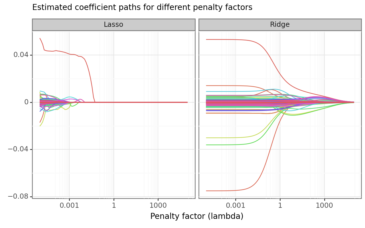
Tune a model
To compute \(\hat\beta_\lambda^\text{Lasso}\) , we simply imposed an arbitrary value for the penalty hyperparameter \(\lambda\). Model tuning is the process of optimally selecting such hyperparameters through cross-validation.
The goal for choosing \(\lambda\) (or any other hyperparameter, e.g., \(\rho\) for the Elastic Net) is to find a way to produce predictors \(\hat{Y}\) for an outcome \(Y\) that minimizes the mean squared prediction error \(\text{MSPE} = E\left( \frac{1}{T}\sum_{t=1}^T (\hat{y}_t - y_t)^2 \right)\). Unfortunately, the MSPE is not directly observable. We can only compute an estimate because our data is random and because we do not observe the entire population.
Obviously, if we train an algorithm on the same data that we use to compute the error, our estimate \(\text{MSPE}\) would indicate way better predictive accuracy than what we can expect in real out-of-sample data. The result is called overfitting.
Cross-validation is a technique that allows us to alleviate this problem. We approximate the true MSPE as the average of many MSPE obtained by creating predictions for \(K\) new random samples of the data, none of them used to train the algorithm \(\frac{1}{K} \sum_{k=1}^K \frac{1}{T}\sum_{t=1}^T \left(\hat{y}_t^k - y_t^k\right)^2\). In practice, this is done by carving out a piece of our data and pretending it is an independent sample. We again divide the data into a training set and a test set. The MSPE on the test set is our measure for actual predictive ability, while we use the training set to fit models with the aim to find the optimal hyperparameter values. To do so, we further divide our training sample into (several) subsets, fit our model for a grid of potential hyperparameter values (e.g., \(\lambda\)), and evaluate the predictive accuracy on an independent sample. This works as follows:
- Specify a grid of hyperparameters
- Obtain predictors \(\hat{y}_i(\lambda)\) to denote the predictors for the used parameters \(\lambda\)
- Compute \[ \text{MSPE}(\lambda) = \frac{1}{K} \sum_{k=1}^K \frac{1}{T}\sum_{t=1}^T \left(\hat{y}_t^k(\lambda) - y_t^k\right)^2 . \tag{11}\] With K-fold cross-validation, we do this computation \(K\) times. Simply pick a validation set with \(M=T/K\) observations at random and think of these as random samples \(y_1^k, \dots, y_{\tilde{T}}^k\), with \(k=1\).
How should you pick \(K\)? Large values of \(K\) are preferable because the training data better imitates the original data. However, larger values of \(K\) will have much higher computation time. scikit-learn provides all required tools to conduct \(K\)-fold cross-validation. We just have to update our model specification. In our case, we specify the penalty factor \(\lambda\) as well as the mixing factor \(\rho\) as free parameters.
For our sample, we consider a time-series cross-validation sample. This means that we tune our models with 20 samples of length five years with a validation period of four years. For a grid of possible hyperparameters, we then fit the model for each fold and evaluate \(\hat{\text{MSPE}}\) in the corresponding validation set. Finally, we select the model specification with the lowest MSPE in the validation set. First, we define the cross-validation folds based on our training data only.
Then, we evaluate the performance for a grid of different penalty values. scikit-learn provides functionalities to construct a suitable grid of hyperparameters with GridSearchCV(). The code chunk below creates a \(10 \times 3\) hyperparameters grid. Then, the method fit() evaluates all the models for each fold.
initial_years = 5
assessment_months = 48
n_splits = int(len(data_manufacturing)/assessment_months) - 1
length_of_year = 12
alphas = np.logspace(-6, 2, 100)

data_folds = TimeSeriesSplit(
  n_splits=n_splits,
  test_size=assessment_months,
  max_train_size=initial_years * length_of_year
)

params = {
  "regressor__alpha": alphas,
  "regressor__l1_ratio": (0.0, 0.5, 1)
}

finder = GridSearchCV(
  lm_pipeline,
  param_grid=params,
  scoring="neg_root_mean_squared_error",
  cv=data_folds
)

finder = finder.fit(
  data_manufacturing, data_manufacturing.get("ret_excess")
)
After the tuning process, we collect the evaluation metrics (the root mean-squared error in our example) to identify the optimal model. Figure 4 illustrates the average validation set’s root mean-squared error for each value of \(\lambda\) and \(\rho\).
validation = (pd.DataFrame(finder.cv_results_)
  .assign(
    mspe=lambda x: -x["mean_test_score"],
    param_regressor__alpha=lambda x: pd.to_numeric(
      x["param_regressor__alpha"], errors="coerce"
    )
  )
)

validation_figure = (
  ggplot(
    validation,
    aes(x="param_regressor__alpha", y="mspe",
        color="param_regressor__l1_ratio",
        shape="param_regressor__l1_ratio",
        group="param_regressor__l1_ratio")
  )
  + geom_point()
  + geom_line()
  + labs(
      x ="Penalty factor (lambda)", y="Root MSPE",
      title="Root MSPE for different penalty factors",
       color="Proportion of Lasso Penalty",
       shape="Proportion of Lasso Penalty"
    )
  + scale_x_log10()
  + guides(linetype="none")
)
validation_figure.show()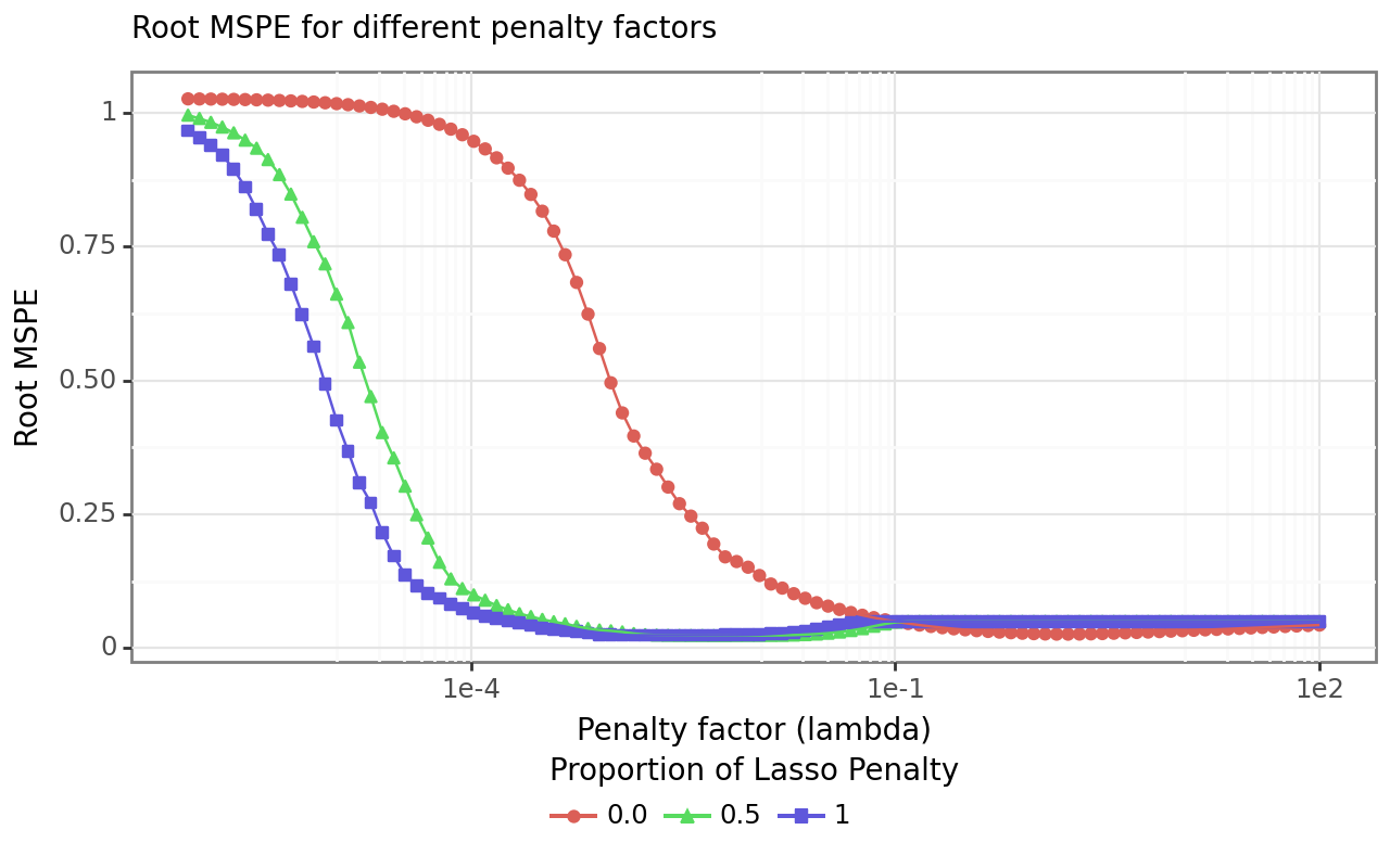
Figure 4 shows that the MSPE drops faster for Lasso and Elastic Net compared to Ridge regressions as penalty factor increases. However, for higher penalty factors, the MSPE for Ridge regressions dips below the others, which both slightly increase again above a certain threshold. Recall that the larger the regularization, the more restricted the model becomes. The best performing model yields a penalty parameter (alpha) of 0.0043 and a mixture factor (\(\rho\)) of 0.5.
Full workflow
Our starting point was the question: Which factors determine industry returns? While Avramov et al. (2023) provide a Bayesian analysis related to the research question above, we choose a simplified approach: To illustrate the entire workflow, we now run the penalized regressions for all ten industries. We want to identify relevant variables by fitting Lasso models for each industry returns time series. More specifically, we perform cross-validation for each industry to identify the optimal penalty factor \(\lambda\).
First, we define the Lasso model with one tuning parameter.
lm_model = Lasso(fit_intercept=False, max_iter=5000)

params = {"regressor__alpha": alphas}

lm_pipeline = Pipeline([
  ("preprocessor", preprocessor),
  ("regressor", lm_model)
])
The following task can be easily parallelized to reduce computing time, but we use a simple loop for ease of exposition.
all_industries = data["industry"].drop_duplicates()

results = []
for industry in all_industries:
  print(industry)
  finder = GridSearchCV(
    lm_pipeline,
    param_grid=params,
    scoring="neg_mean_squared_error",
    cv=data_folds
  )

  finder = finder.fit(
    data.query("industry == @industry"),
    data.query("industry == @industry").get("ret_excess")
  )
  results.append(
    pd.DataFrame(finder.best_estimator_.named_steps.regressor.coef_ != 0)
  )

selected_factors = (
  pd.DataFrame(
    lm_pipeline[:-1].get_feature_names_out(),
    columns=["variable"]
  )
  .assign(variable = lambda x: (
    x["variable"].str.replace("factor_|ff_|q_|macro_",""))
  )
  .assign(**dict(zip(all_industries, results)))
  .melt(id_vars="variable", var_name ="industry")
  .query("value == True")
)
What has just happened? In principle, exactly the same as before but instead of computing the Lasso coefficients for one industry, we did it for ten sequentially. Now, we just have to do some housekeeping and keep only variables that Lasso does not set to zero. We illustrate the results in a heat map in Figure 5.
selected_factors_figure = (
  ggplot(
    selected_factors,
    aes(x="variable", y="industry")
  )
  + geom_tile()
  + labs(x="", y="", title="Selected variables for different industries")
  + coord_flip()
  + scale_x_discrete(limits=reversed)
  + theme(axis_text_x=element_text(rotation=70, hjust=1), figure_size=(6.4, 6.4))
)
selected_factors_figure.show()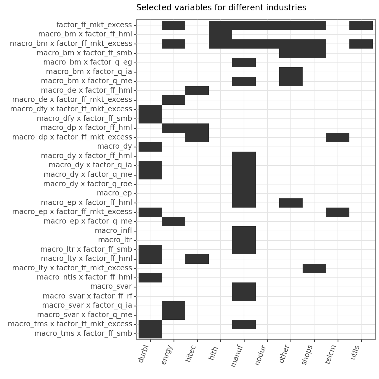
The heat map in Figure 5 conveys two main insights: first, we see that many factors, macroeconomic variables, and interaction terms are not relevant for explaining the cross-section of returns across the industry portfolios. In fact, only factor_ff_mkt_excess and its interaction with macro_bm a role for several industries. Second, there seems to be quite some heterogeneity across different industries. While barely any variable is selected by Lasso for Utilities, many factors are selected for, e.g., Durable and Manufacturing, but the selected factors do not necessarily coincide. In other words, there seems to be a clear picture that we do not need many factors, but Lasso does not provide a factor that consistently provides pricing abilities across industries.
Key Takeaways
- The
scikit-learnframework in Python enables a clean, modular workflow for pre-processing financial data, fitting models, and tuning hyperparameters through cross-validation. - Lasso regression is especially useful in high-dimensional settings, as it performs automatic variable selection by setting irrelevant coefficients to zero, offering insights into which factors truly matter.
- Applying these methods to real-world data shows that only a few factors consistently explain industry portfolio returns, and the relevant predictors vary across industries.
- The analysis demonstrates practical tools to handle overfitting, model complexity, and interpretability in empirical asset pricing.
Exercises
- Write a function that requires three inputs, namely,
y(a \(T\) vector),X(a \((T \times K)\) matrix), andlambdaand then returns the Ridge estimator (a \(K\) vector) for a given penalization parameter \(\lambda\). Recall that the intercept should not be penalized. Therefore, your function should indicate whether \(X\) contains a vector of ones as the first column, which should be exempt from the \(L_2\) penalty. - Compute the \(L_2\) norm (\(\beta'\beta\)) for the regression coefficients based on the predictive regression from the previous exercise for a range of \(\lambda\)’s and illustrate the effect of penalization in a suitable figure.
- Now, write a function that requires three inputs, namely,
y(a \(T\) vector),X(a \((T \times K)\) matrix), and \(\lambda\) and then returns the Lasso estimator (a \(K\) vector) for a given penalization parameter \(\lambda\). Recall that the intercept should not be penalized. Therefore, your function should indicate whether \(X\) contains a vector of ones as the first column, which should be exempt from the \(L_1\) penalty. - After you understand what Ridge and Lasso regressions are doing, familiarize yourself with the
glmnetpackage’s documentation. It is a thoroughly tested and well-established package that provides efficient code to compute the penalized regression coefficients for Ridge and Lasso and for combinations, commonly called Elastic Nets.
References
Avramov, Doron, Si Cheng, Lior Metzker, and Stefan Voigt. 2023. “Integrating factor models.” The Journal of Finance 78 (3): 1593–1646. https://doi.org/10.1111/jofi.13226.
Cochrane, John H. 2009. Asset pricing (revised edition). Princeton University Press.
———. 2011. “Presidential address: Discount rates.” The Journal of Finance 66 (4): 1047–1108. https://doi.org/10.1111/j.1540-6261.2011.01671.x.
De Prado, Marcos Lopez. 2018. Advances in financial machine learning. John Wiley & Sons. https://doi.org/10.5555/3217448.
Dixon, Matthew F., Igor Halperin, and Paul Bilokon. 2020. Machine learning in finance. Springer.
Easley, David, Marcos de Prado, Maureen O’Hara, and Zhibai Zhang. 2020. “Microstructure in the machine age.” Review of Financial Studies 34 (7): 3316–63. https://doi.org/10.1093/rfs/hhaa078.
Fama, Eugene F., and Kenneth R. French. 1992. “The cross-section of expected stock returns.” The Journal of Finance 47 (2): 427–65. https://doi.org/2329112.
———. 1993. “Common risk factors in the returns on stocks and bonds.” Journal of Financial Economics 33 (1): 3–56. https://doi.org/10.1016/0304-405X(93)90023-5.
Gareth, James, Witten Daniela, Hastie Trevor, and Tibshirani Robert. 2013. An introduction to statistical learning: With applications in R. Springer.
Harvey, Campbell R. 2017. “Presidential address: The scientific outlook in financial economics.” The Journal of Finance 72 (4): 1399–1440. https://doi.org/10.1111/jofi.12530.
Harvey, Campbell R., Yan Liu, and Heqing Zhu. 2016. “\(\ldots\) and the cross-section of expected returns.” Review of Financial Studies 29 (1): 5–68. https://doi.org/10.1093/rfs/hhv059.
Hastie, Trevor, Robert Tibshirani, and Jerome Friedman. 2009. The elements of statistical learning: Data mining, inference and prediction. 2nd ed. Springer. https://hastie.su.domains/ElemStatLearn/.
Hoerl, Arthur E., and Robert W. Kennard. 1970. “Ridge regression: Applications to nonorthogonal problems.” Technometrics 12 (1): 69–82. https://doi.org/1267352.
Hou, Kewei, Chen Xue, and Lu Zhang. 2014. “Digesting anomalies: An investment approach.” Review of Financial Studies 28 (3): 650–705. https://doi.org/10.1093/rfs/hhu068.
———. 2020. “Replicating anomalies.” Review of Financial Studies 33 (5): 2019–2133. https://doi.org/10.1093/rfs/hhy131.
Mclean, R. David, and Jeffrey Pontiff. 2016. “Does academic research destroy stock return predictability?” The Journal of Finance 71 (1): 5–32. https://doi.org/10.1111/jofi.12365.
Mullainathan, Sendhil, and Jann Spiess. 2017. “Machine learning: An applied econometric approach.” Journal of Economic Perspectives 31 (2): 87–106. https://doi.org/10.1257/jep.31.2.87.
Nagel, Stefan. 2021. Machine learning in asset pricing. Princeton University Press.
Pedregosa, F., G. Varoquaux, A. Gramfort, V. Michel, B. Thirion, O. Grisel, M. Blondel, et al. 2011. “Scikit-Learn: Machine Learning in Python.” Journal of Machine Learning Research 12: 2825–30.
Tibshirani, Robert. 1996. “Regression shrinkage and selection via the LASSO.” Journal of the Royal Statistical Society. Series B (Methodological) 58 (1): 267–88. http://www.jstor.org/stable/2346178.
Welch, Ivo, and Amit Goyal. 2008. “A comprehensive look at the empirical performance of equity premium prediction.” Review of Financial Studies 21 (4): 1455–1508. https://doi.org/10.1093/rfs/hhm014.
Zou, Hui, and Trevor Hastie. 2005. “Regularization and variable selection via the elastic net.” Journal of the Royal Statistical Society. Series B (Statistical Methodology) 67 (2): 301–20. https://www.jstor.org/stable/3647580.