Modern Portfolio Theory

Note

You are reading Tidy Finance with Python. You can find the equivalent chapter for the sibling Tidy Finance with R here.

In the previous chapter, we show how to download and analyze stock market data with figures and summary statistics. Now, we move to a typical question in finance: How should an investor allocate their wealth across assets that differ in expected returns, variance, and correlations to optimize their portfolio’s performance? Modern Portfolio Theory (MPT), introduced by Markowitz (1952), revolutionized the way how we think about such investment decisions by formalizing the trade-off between risk and expected return. Markowitz’s framework laid the foundation for much of modern finance, also earning him the Sveriges Riksbank Prize in Economic Sciences in 1990.

MPT relies on the fact that portfolio risk depends on individual asset volatilities as well as on the correlations between asset returns. This insight highlights the power of diversification: Combining assets with low or negative correlations with a given portfolio reduces the overall portfolio risk. This principle is often illustrated with the analogy of a fruit basket: If all you have are apples and they spoil, you lose everything. With a variety of fruits, some fruits may spoil, but others will stay fresh.

At the heart of MPT is mean-variance analysis, which evaluates portfolios based on two dimensions: expected return and risk, defined as the variance of the portfolio returns. By balancing these two components, investors can construct portfolios that either maximize their expected return for a given level of risk or minimize their taken risk for a desired level of return. In this chapter, we first derive the optimal portfolio decisions and implement the mean-variance approach in R.

We use the following packages throughout this chapter:

import pandas as pd
import numpy as np
import yfinance as yf

from plotnine import *
from mizani.formatters import percent_format
from adjustText import adjust_text

We introduce the adjustText package for adding text labels to the figures in this chapter (Flyamer 2024).

The Asset Universe

Suppose that \(N\) different risky assets are available to the investor. Each asset \(i\) delivers expected returns \(\mu_i\), representing the anticipated profit from holding the asset for one period. The investor can allocate their wealth across these assets by choosing the portfolio weights \(\omega_i\) for each asset \(i\). We impose that the portfolio weights sum up to one to ensure that the investor is fully invested. There is no outside option, such as keeping your money under a mattress. The overarching question of this chapter is: How should the investor allocate their wealth across these assets to optimize their portfolio’s performance?

According to Markowitz (1952), portfolio selection involves two stages: First, forming expectations about future security performance based on observations and experience. Second, using these expectations to choose a portfolio. In practice, these two steps cannot be separated. You need historical data or other considerations to generate estimates of the distribution of future returns. Only then can one proceed proceed to optimal decision-making conditional on your estimation.

To keep things conceptually simple, we focus on the latter part for now and assume that the actual distribution of the asset returns is known. In later chapters, we discuss the issues that arise once we take estimation uncertainty into account. To provide some meaningful illustrations, we rely on historical data to compute reasonable proxies for the expected returns and the variance-covariance of the assets returns, but we will work under the assumption that these are the true parameters of the return distribution.

Thus, leveraging the approach introduced in Working with Stock Returns, we download the constituents of the Dow Jones Industrial Average as an example portfolio as well as their daily adjusted close prices.

import ssl
ssl._create_default_https_context = ssl._create_unverified_context

url = ("https://www.ssga.com/us/en/institutional/etfs/library-content/"
       "products/fund-data/etfs/us/holdings-daily-us-en-dia.xlsx")

symbols = (pd.read_excel(url, skiprows=4, nrows=30)
  .get("Ticker")
  .tolist()
)

ssl._create_default_https_context = ssl.create_default_context

prices_daily = (yf.download(
    tickers=symbols, 
    start="2000-01-01", 
    end="2023-12-31", 
    progress=False,
    auto_adjust=False,
    multi_level_index=False
  ))

prices_daily = (prices_daily
  .stack()
  .reset_index(level=1, drop=False)
  .reset_index()
  .rename(columns={"Ticker": "symbol", "Date": "date", "Adj Close": "adjusted"})
)

To have a stable stock universe and to keep the analysis simple, we ensure that all stocks were traded over the whole sample period:

prices_daily = (prices_daily
  .groupby("symbol")
  .apply(lambda x: x.assign(counts=x["adjusted"].dropna().count()))
  .reset_index(drop=True)
  .query("counts == counts.max()")
)

We compute the sample average returns as \(\mu_i = \frac{1}{T} \sum_{t=1}^{T} r_{i,t},\) where \(r_{i,t}\) is the return of asset \(i\) in period \(t\), and \(T\) is the total number of periods. As noted above, we treat the vector \(\mu = (\mu_1, ...,\mu_N)^\prime\) as the true expected return of the assets. For simplicity and easier interpretation, we focus on monthly returns going forward.

returns_monthly = (prices_daily
  .assign(
    date=prices_daily["date"].dt.to_period("M").dt.to_timestamp()
  )
  .groupby(["symbol", "date"], as_index=False)
  .agg(adjusted=("adjusted", "last"))
  .assign(
    ret=lambda x: x.groupby("symbol")["adjusted"].pct_change()
  )
)

Individual asset risk in MPT is typically quantified using variance (i.e., \(\sigma^2_i\)) or volatilities (i.e., \(\sigma_i\)).¹ We suppose that the true volatilities of the assets are given by the sample standard deviation \(\sigma_i = \sqrt{\frac{1}{T-1} \sum_{t=1}^{T} (r_{i,t} - \mu_i)^2}.\)

We compute the sample standard deviation for each asset by using the std() function.

assets = (returns_monthly
  .groupby("symbol", as_index=False)
  .agg(
    mu=("ret", "mean"),
    sigma=("ret", "std")
  )
)

We can illustrate the resulting distribution of the asset returns in Figure 1, showing the volatility on the horizontal axis and the expected return on the vertical axis.

(
  ggplot(assets, aes(x="sigma", y="mu", label="symbol"))
  + geom_point()
  + geom_text(adjust_text={"arrowprops": {"arrowstyle": "-"}})
  + scale_x_continuous(labels=percent_format())
  + scale_y_continuous(labels=percent_format())
  + labs(
      x="Volatility", y="Expected return",
      title="Expected returns and volatilities of Dow Jones index constituents"
  )
)

Figure 1: Expected returns and volatilities based on monthly returns adjusted for dividend payments and stock splits.

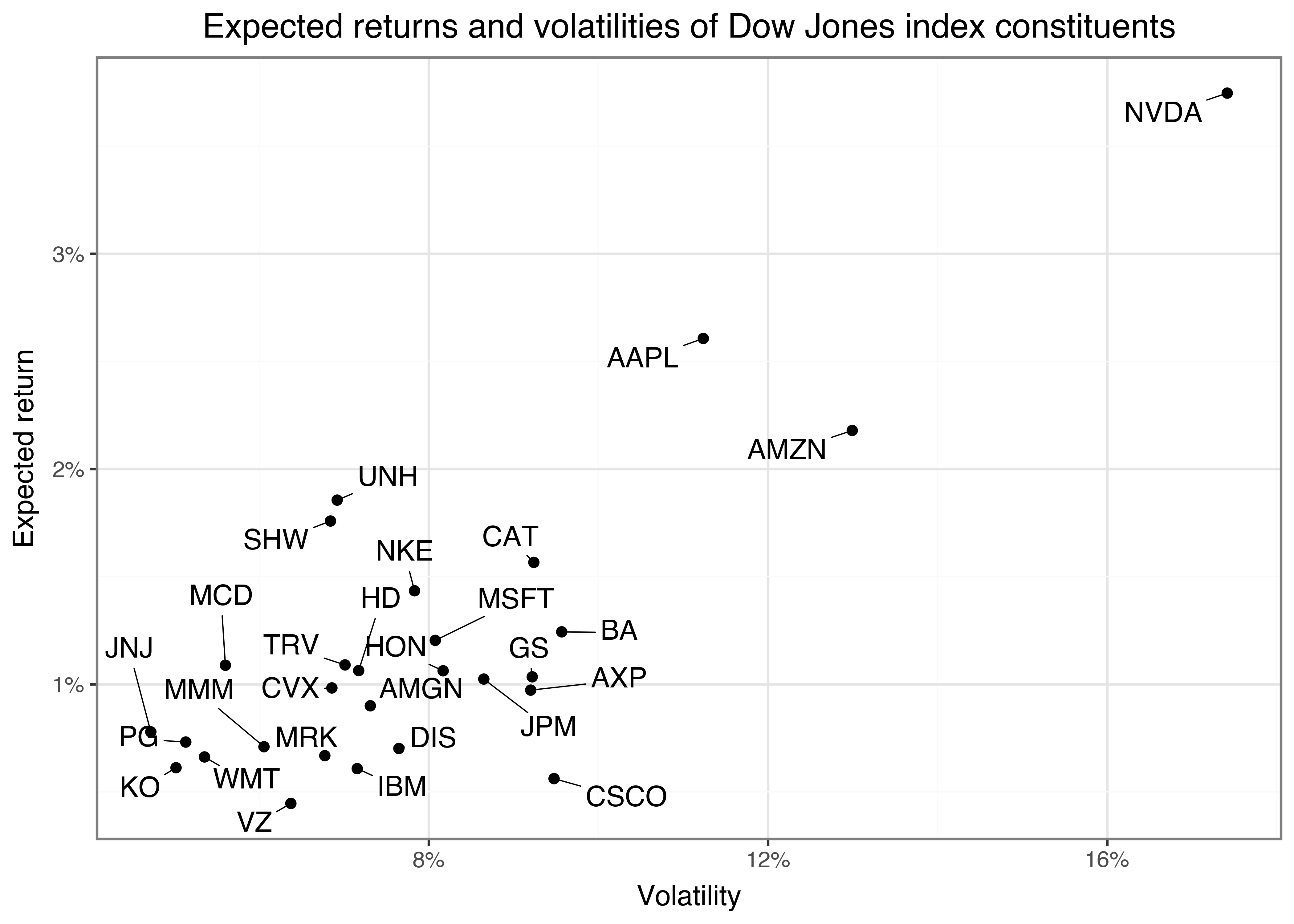
As highlighted above, a key innovation of MPT is to consider interactions between assets. The variance-covariance matrix collects this information. We assume that the variance-covariance matrix \(\Sigma\) of the returns is given by the sample covariance:

\[\sigma_{i,j} = \frac{1}{T-1} \sum_{t=1}^{T} (r_{i,t} - \mu_i)(r_{j,t} - \mu_j)\]

The interpretation is straightforward: While a positive covariance between assets indicates that these assets tend to move in the same direction, a negative covariance indicates that the assets move in opposite directions.

We can use the cov() function that takes a matrix of returns as inputs. We thus need to transform the returns from a data frame into a \((T \times N)\) matrix with one column for each of the \(N\) symbols and one row for each of the \(T\) trading days. We achieve this by using pivot_wider() with the new column names from the symbol-column and setting the values to ret.

returns_wide = (returns_monthly
  .pivot(index="date", columns="symbol", values="ret")
  .reset_index()
)

sigma = (returns_wide
  .drop(columns=["date"])
  .cov()
)

Figure Figure 2 illustrates the resulting variance-covariance matrix.

sigma_long = (sigma
  .reset_index()
  .melt(id_vars="symbol", var_name="symbol_b", value_name="value")
)

sigma_long["symbol_b"] = pd.Categorical(
  sigma_long["symbol_b"], 
  categories=sigma_long["symbol_b"].unique()[::-1],
  ordered=True
)

(
  ggplot(sigma_long, aes(x="symbol", y="symbol_b", fill="value"))
  + geom_tile()
  + labs(
      x="", y="", fill="(Co-)Variance",
      title="Variance-covariance matrix of Dow Jones index constituents"
    )
  + scale_fill_continuous(labels=percent_format())
  + theme(axis_text_x=element_text(angle=45, hjust=1))
)

Figure 2: Variances and covariances based on monthly returns adjusted for dividend payments and stock splits.

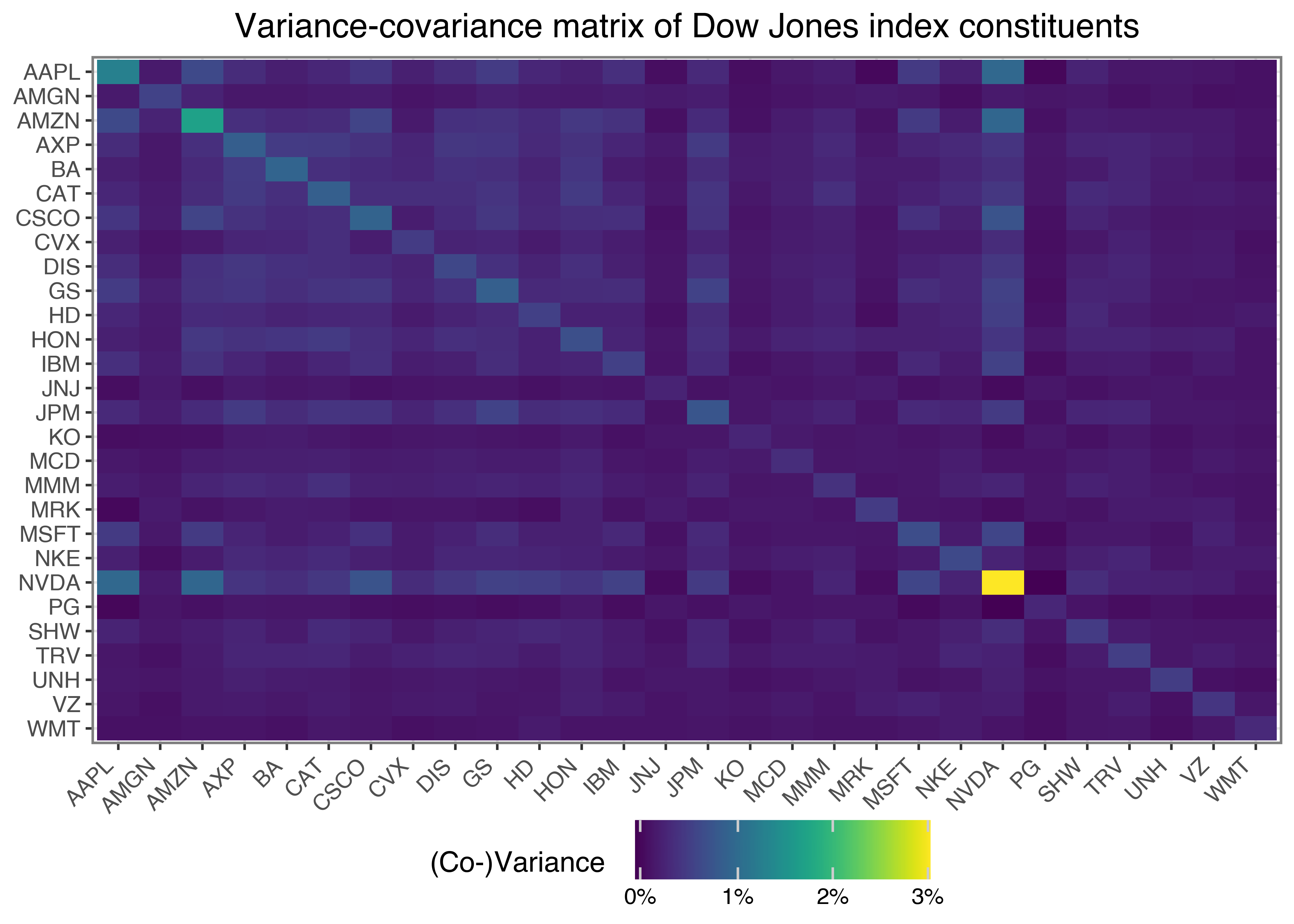
The Minimum-Variance Framework

Suppose now the investor allocates their wealth in a portfolio given by the weight vector \(\omega\). The resulting portfolio returns \(\omega^\prime r\) have an expected return \(\mu_\omega = \omega^{\prime}\mu = \sum_{i=1}^N \omega_i \mu_i\). The variance of the portfolio returns is \(\sigma^2_\omega = \omega^{\prime}\Sigma\omega = \sum_{i=1}^{N} \sum_{j=1}^{N} \omega_i \omega_j \sigma_{ij}\) where \(\omega_i\) and \(\omega_j\) are the weights of assets \(i\) and \(j\) in the portfolio, respectively, and \(\sigma_{ij}\) is the covariance between returns of assets \(i\) and \(j\).

We first consider an investor who wants to invest in a portfolio that delivers the lowest possible variance as a reference point. Thus, the optimization problem of the minimum-variance investor is given by

\[\min_{\omega_1, ... \omega_n} \sum_{i=1}^{n} \sum_{j=1}^{n} \omega_i \omega_j \sigma_{ij} = \min_\omega \omega^{\prime}\Sigma\omega.\]

While staying fully invested across all available assets \(N\), \(\sum_{i=1}^{N} \omega_i = 1\). The analytical solution for the minimum-variance portfolio is

\[\omega_\text{mvp} = \frac{\Sigma^{-1}\iota}{\iota^{\prime}\Sigma^{-1}\iota},\]

where \(\iota\) is a vector of 1’s and \(\Sigma^{-1}\) is the inverse of the variance-covariance matrix \(\Sigma\). See Proofs in the Appendix for details on the derivation. In the following code chunk, we calculate the weights of the minimum-variance portfolio:

iota = np.ones(sigma.shape[0])
sigma_inv = np.linalg.inv(sigma.values)
omega_mvp = (sigma_inv @ iota) / (iota @ sigma_inv @ iota)

Figure Figure 3 shows the resulting portfolio weights.

assets = assets.assign(omega_mvp=omega_mvp)

assets["symbol"] = pd.Categorical(
  assets["symbol"],
  categories=assets.sort_values("omega_mvp")["symbol"],
  ordered=True
)

(
  ggplot(assets,
         aes(y="omega_mvp", x="symbol", fill="omega_mvp>0"))
  + geom_col()
  + coord_flip()
  + scale_y_continuous(labels=percent_format())
  + labs(x="", y="",
       title="Minimum-variance portfolio weights")
  + theme(legend_position="none")
)

Figure 3: Weights are based on historical moments of monthly returns adjusted for dividend payments and stock splits.

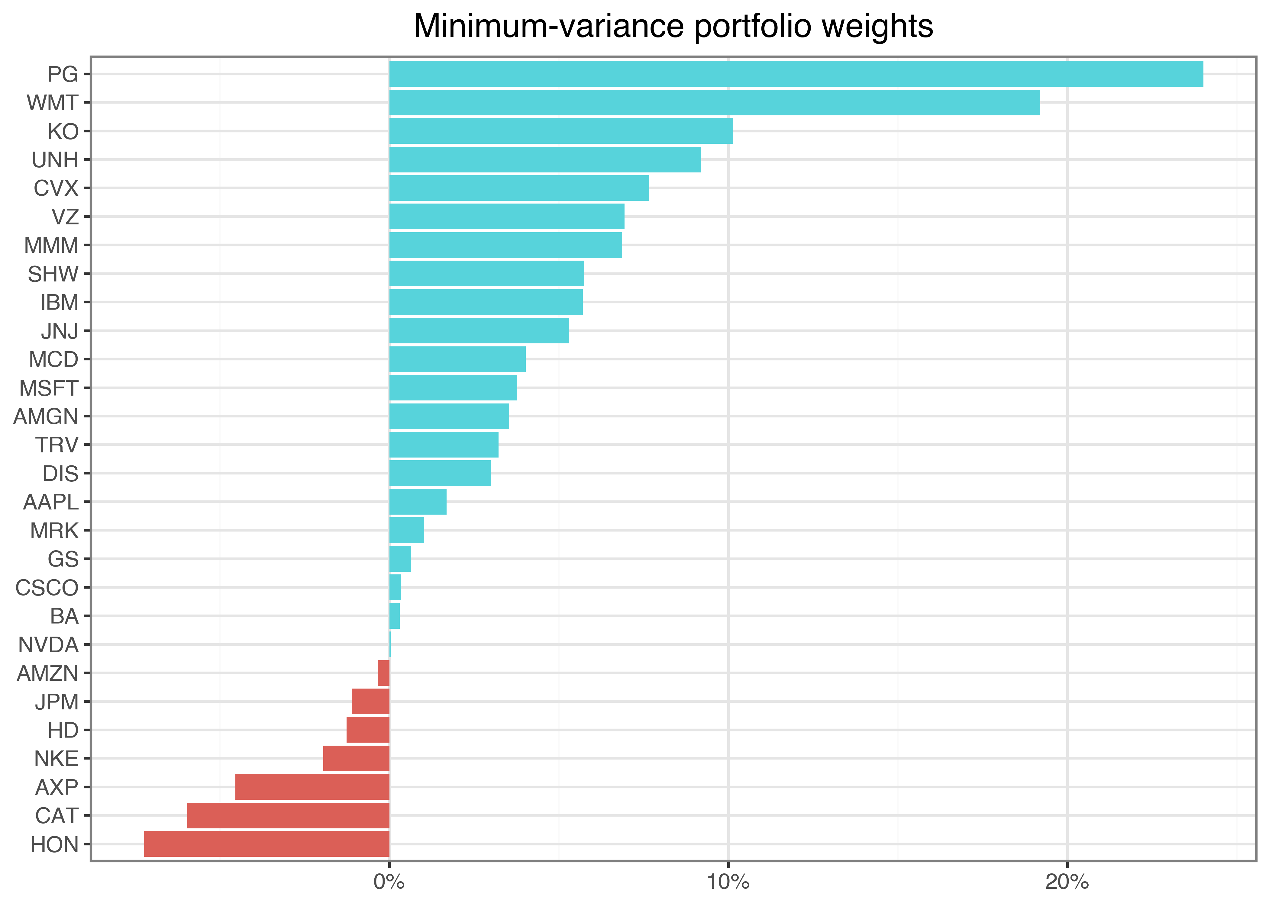
Before we move on to other portfolios, we collect the return and volatility of the minimum-variance portfolio in a data frame:

mu = assets["mu"].values
mu_mvp = omega_mvp @ mu
sigma_mvp = np.sqrt(omega_mvp @ sigma.values @ omega_mvp)
summary_mvp = pd.DataFrame({
  "mu": [mu_mvp],
  "sigma": [sigma_mvp],
  "type": ["Minimum-Variance Portfolio"]
})
summary_mvp

	mu	sigma	type
0	0.008356	0.032144	Minimum-Variance Portfolio

Efficient Portfolios

In many instances, earning the lowest possible variance may not be the desired outcome. Instead, we generalize the concept of efficient portfolios, where, in addition to minimizing portfolio variance, the investor aims to earn a minimum expected return \(\omega^{\prime}\mu \geq \bar{\mu}.\) In other words, when \(\bar\mu\geq \omega_\text{mvp}^{\prime}\mu\), the investor is willing to accept a higher portfolio variance in return for earning a higher expected return.

Suppose, for instance, the investor wants to earn at least the historical average return of the asset that delivered the highest average returns in the past:

mu_bar = assets["mu"].max()

Formally, the optimization problem is given by

\[\min_\omega \omega^{\prime}\Sigma\omega \text{ s.t. } \omega^{\prime}\iota = 1 \text{ and } \omega^{\prime}\mu\geq\bar\mu.\]

The analytic solution for the efficient portfolio can be derived as:

\[\omega_{efp} = \frac{\lambda^*}{2}\left(\Sigma^{-1}\mu -\frac{D}{C}\Sigma^{-1}\iota \right),\]

where \(\lambda^* = 2\frac{\bar\mu - D/C}{E-D^2/C}\), \(C = \iota'\Sigma^{-1}\iota\), \(D=\iota'\Sigma^{-1}\mu\), and \(E=\mu'\Sigma^{-1}\mu\). For details, we again refer to the Proofs in the Appendix.

The code below implements the analytic solution to this optimization problem and collects the resulting portfolio return and risk in a data frame.

C = iota @ sigma_inv @ iota
D = iota @ sigma_inv @ mu
E = mu @ sigma_inv @ mu
lambda_tilde = 2 * (mu_bar - D / C) / (E - (D ** 2) / C)
omega_efp = omega_mvp + (lambda_tilde / 2) * (sigma_inv @ mu - D * omega_mvp)
mu_efp = omega_efp @ mu
sigma_efp = np.sqrt(omega_efp @ sigma.values @ omega_efp)

summary_efp = pd.DataFrame({
  "mu": [mu_efp],
  "sigma": [sigma_efp],
  "type": ["Efficient Portfolio"]
})

Figure Figure 4 shows the average return and volatility of the minimum-variance and the efficient portfolio relative to the index constituents. As expected, the efficient portfolio has a higher expected return at the cost of higher volatility compared to the minimum-variance portfolio.

summaries = pd.concat(
  [assets, summary_mvp, summary_efp], ignore_index=True
)

(
  ggplot(summaries, 
         aes(x="sigma", y="mu"))
  + geom_point(
      data=summaries.query("type.isna()")
    )
  + geom_point(
      data=summaries.query("type.notna()"), color="#F21A00", size=3
    )
  + geom_label(aes(label="type"), adjust_text={"arrowprops": {"arrowstyle": "-"}})
  + scale_x_continuous(labels=percent_format())
  + scale_y_continuous(labels=percent_format())
  + labs(
      x="Volatility", y="Expected return",
      title="Efficient & minimum-variance portfolios"
    ) 
)

Figure 4: The big dots indicate the location of the minimum-variance and the efficient portfolio that delivers the expected return of the stock with the higehst return, respectively. The small dots indicate the location of the individual constituents.

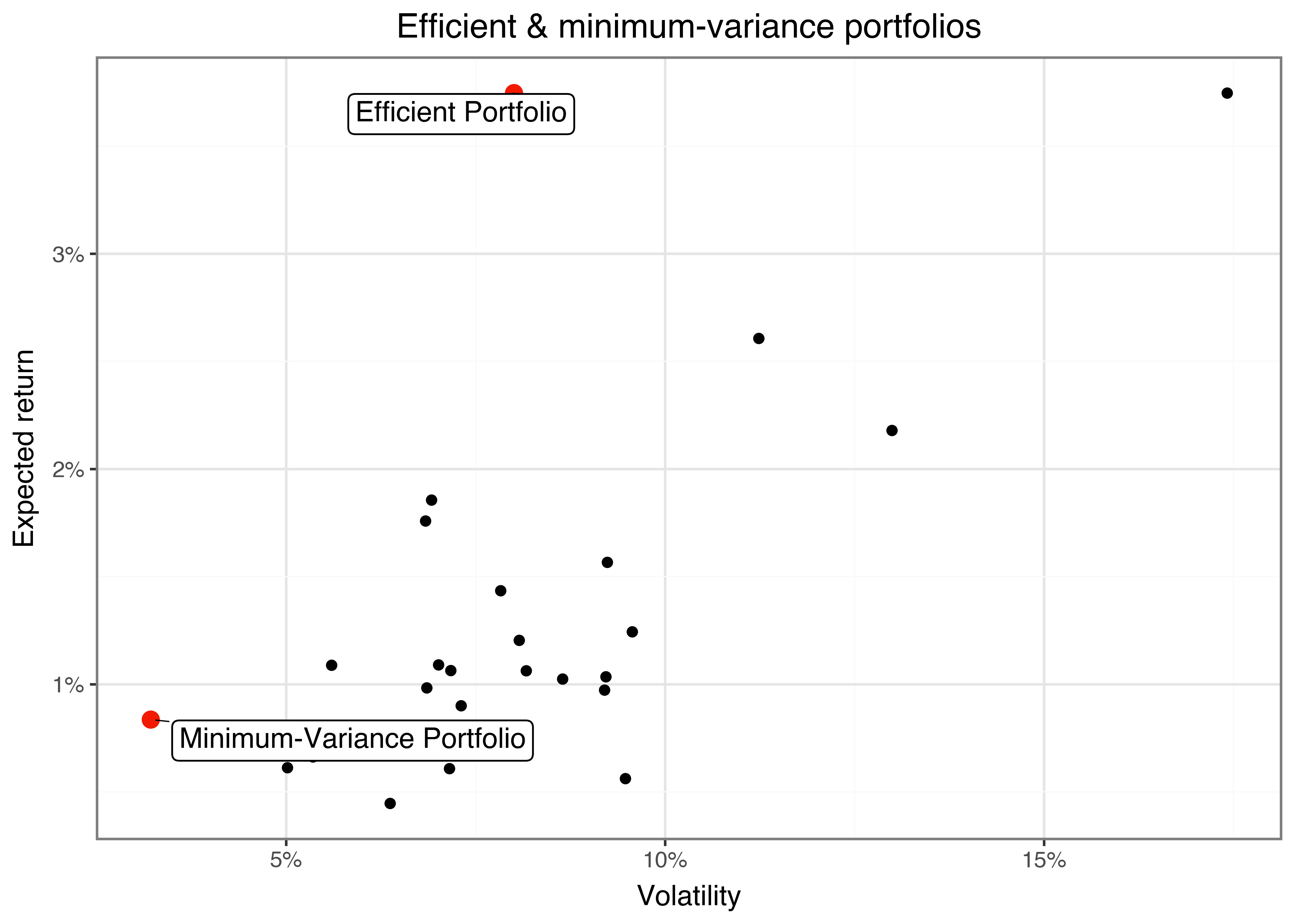
The figure illustrates the substantial diversification benefits: Instead of allocating all wealth into one asset that delivered a high average return in the past (at a substantial volatility), the efficient portfolio promises exactly the same expected returns but at a much lower volatility.

It should be noted that the level of desired returns \(\bar\mu\) reflects the risk-aversion of the investor. Less risk-averse investors may require a higher level of desired returns. In contrast, more risk-averse investors may only choose \(\bar\mu\) closer to the expected return of the minimum-variance portfolio. Very often, the mean-variance framework is instead derived as the optimal decision framework of an investor with a mean-variance utility function with a coefficient of relative risk aversion \(\gamma\). In the Proofs in the Appendix, we show that there is a one-to-one mapping from \(\gamma\) to the desired level of expected returns \(\bar\mu\), which implies that the resulting efficient portfolios are equivalent and do not depend on the way the optimization problem is formulated.

The Efficient Frontier

The set of portfolios that satisfies the condition that no other portfolio exists with a higher expected return for a given level of volatility is called the efficient frontier, see, e.g., Merton (1972). . To derive the portfolios that span the efficient frontier, the mutual fund separation theorem proves very helpful. In short, the theorem states that as soon as we have two efficient portfolios (such as the minimum-variance portfolio \(\omega_\text{mvp}\) and the efficient portfolio for a higher required level of expected returns \(\omega_\bar\mu\), we can characterize the entire efficient frontier by combining these two portfolios. That is, any linear combination of the two portfolio weights will again represent an efficient portfolio. In other words, the efficient frontier can be characterized by the following equation:

\[\omega_{a\mu_1 + (1-a)\mu_2} = a \cdot \omega_{\mu_1} + (1-a) \cdot\omega_{\mu_2},\]

where \(a\) is a scalar between 0 and 1, \(\omega_{\mu_i}\) is an efficient portfolio that delivers the expected return \(\mu_i\). It is straightforward to prove the theorem. Consider the analytical solution for the efficient portfolio, which delivers expected returns \(\mu_i\), implying:

\[a \cdot \omega_{\mu_1} + (1-a) \cdot\omega_{\mu_2} = \left(\frac{a\mu_1 + (1-a)\mu_2- D/C }{E-D^2/C}\right)\left(\Sigma^{-1}\mu -\frac{D}{C}\Sigma^{-1}\iota \right),\]

which corresponds to the efficient portfolio earning \(a\mu_1 + (1-a)\mu_2\) in expectation.

The code below implements the construction of this efficient frontier, which characterizes the highest expected return achievable at each level of risk.

efficient_frontier = (
  pd.DataFrame({
    "a": np.arange(-1, 2.01, 0.01)
  })
  .assign(
    omega=lambda x: x["a"].map(lambda x: x * omega_efp + (1 - x) * omega_mvp)
  )
  .assign(
    mu=lambda x: x["omega"].map(lambda x: x @ mu),
    sigma=lambda x: x["omega"].map(lambda x: np.sqrt(x @ sigma @ x))
  )
)

Finally, it is simple to visualize the efficient frontier alongside the two efficient portfolios in a figure using ggplot (see Figure 5). We also add the individual stocks in the same plot.

summaries = pd.concat(
  [summaries, efficient_frontier], ignore_index=True
)

(
  ggplot(summaries, 
         aes(x="sigma", y="mu"))
  + geom_point(
      data = summaries.query("type.isna()")
    )
  + geom_point(
      data = summaries.query("type.notna()"), color="#F21A00", size=3
    )
  + geom_label(aes(label="type"), adjust_text={"arrowprops": {"arrowstyle": "-"}})
  + scale_x_continuous(labels=percent_format())
  + scale_y_continuous(labels=percent_format())
  + labs(
      x="Volatility", y="Expected return",
      title="Efficient & minimum-variance portfolios"
    ) 
)

Figure 5: The big dots indicate the location of the minimum-variance and the efficient portfolio that delivers three times the expected return of the minimum-variance portfolio, respectively. The small dots indicate the location of the individual constituents.

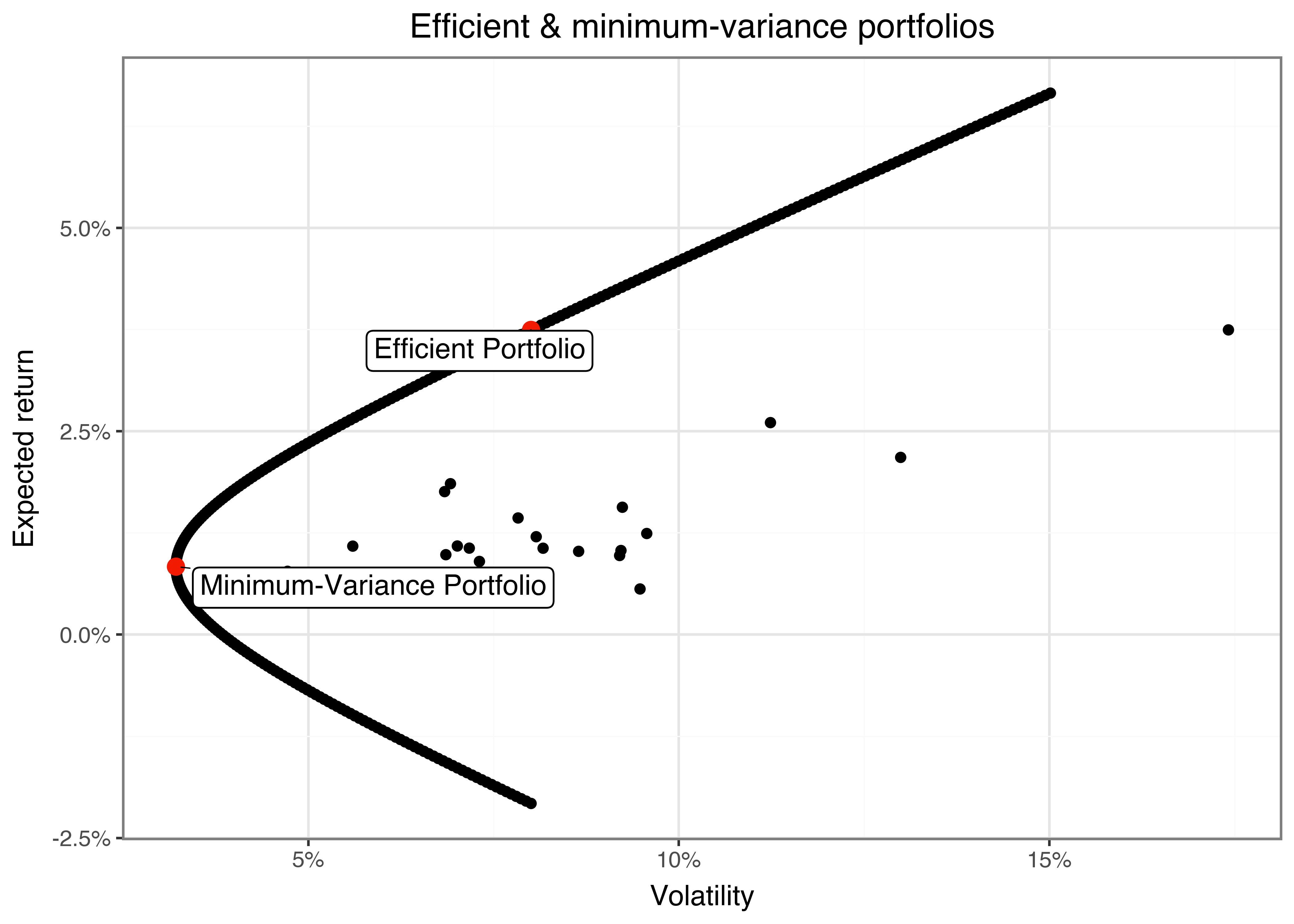
Key Takeaways

The mean-variance framework is a cornerstone of modern finance, emphasizing the trade-off between risk and return. The key insights from this chapter are:

• Mean-variance optimization balances expected returns against expected portfolio risk.
• Portfolio risk depends on both volatilities and correlations between assets.
• The minimum-variance portfolio achieves the lowest possible risk for a given set of assets.
• Efficient portfolios maximize expected return for each level of risk.

Exercises

1. We restricted our sample to all assets trading every day since 2000-01-01. Discuss why this restriction might introduce survivorship bias and how it could affect inferences about future expected portfolio performance.
2. The efficient frontier characterizes portfolios with the highest expected return for different levels of risk. Identify the portfolio with the highest expected return per unit of standard deviation (risk). Which famous performance measure corresponds to the ratio of average returns to standard deviation?
3. Analyze how varying the correlation coefficients between asset returns influences the shape of the efficient frontier. Use hypothetical data for a small number of assets to visualize and interpret these changes.

References

Flyamer, Ilya. 2024. “adjustText.” https://pypi.org/project/adjustText/.

Markowitz, Harry. 1952. “Portfolio selection.” The Journal of Finance 7 (1): 77–91. https://doi.org/10.1111/j.1540-6261.1952.tb01525.x.

Merton, Robert C. 1972. “An analytic derivation of the efficient portfolio frontier.” Journal of Financial and Quantitative Analysis 7 (4): 1851–72. https://doi.org/10.2307/2329621.

Footnotes

1. Alternative approaches include value-at-risk, expected shortfall, or higher-order moments such as skewness and kurtosis.