Discounted Cash Flow Analysis

Note

You are reading Tidy Finance with R. You can find the equivalent chapter for the sibling Tidy Finance with Python here.

In this chapter, we address a fundamental question: What is the value of a company? Company valuation is a critical tool that helps us determine the economic value of a business. Understanding a company’s value is essential, whether it is for investment decisions, mergers and acquisitions, or financial reporting. Valuation is not just about assigning a number, as it is also a framework for making informed decisions. For example, investors use valuation to identify whether a stock is under- or overvalued, and companies rely on valuation for strategic decisions, like pricing an acquisition or preparing for an IPO.

Company valuation methods broadly fall into three categories:

• Market-based approaches compare companies using relative metrics like Price-to-Earnings ratios.
• Asset-based methods focus on the net value of a company’s tangible and intangible assets.
• Income-based techniques value companies based on their ability to generate future cash flows.

We focus on Discounted Cash Flow (DCF) analysis, an income-based approach, because it captures three crucial aspects of valuation: First, DCF explicitly accounts for the time value of money - the principle that a dollar today is worth more than a dollar in the future. By discounting future cash flows to present value with the appropriate discount rate, we incorporate both time preferences and risk. Second, DCF is inherently forward-looking, making it particularly suitable for companies where historical performance may not reflect future potential. This characteristic is especially relevant when valuing growth companies or analyzing new business opportunities. Third, DCF analysis is flexible enough to accommodate various business models and capital structures, making it applicable across different industries and company sizes.

In our exposition of the DCF valuation framework, we focus on its three key components:

• Free Cash Flow (FCF) forecasts represent the expected future cash available for distribution to investors after accounting for operating expenses, taxes, and investments.
• Terminal value captures the company’s value beyond the explicit forecast period, often representing a significant portion of the total valuation.
• Discount rate, typically the Weighted Average Cost of Capital (WACC), adjusts future cash flows to present value by incorporating risk and capital structure considerations.

We make a few simplifying assumptions due to the diverse nature of businesses, which a simple model cannot cover. After all, there are entire textbooks written just on valuation. In particular, we assume that firms only conduct operating activities (i.e., financial statements do not include non-operating items), implying that firms do not own any assets that do not produce operating cash flows. Otherwise, you must value these non-operating activities separately for many real-world examples.

In this chapter, we rely on the following packages to build a simple DCF analysis:

library(tidyverse)
library(tidyfinance)
library(scales)
library(fmpapi)

Tip

The fmpapi package is developed by Christoph Scheuch and is not sponsored by or affiliated with FMP. However, you can get 15% off your FMP subscription by using this affiliate link. By signing up through this link, you also support the development of this package at no extra cost to you.

Prepare Data

Before we can perform a DCF analysis, we need historical financial data to inform our forecasts. We use the Financial Modeling Prep (FMP) API to download financial statements. The fmpapi package provides a convenient interface for accessing this data in a tidy format.

symbol <- "MSFT"

income_statements <- fmp_get(
  "income-statement", symbol, list(period = "annual", limit = 5)
)
cash_flow_statements <- fmp_get(
  "cash-flow-statement", symbol, list(period = "annual", limit = 5)
)

Our analysis centers on Free Cash Flow (FCF), which represents the cash available to all investors after the company has covered its operational needs and capital investments. We calculate FCF using the following formula:

\[\text{FCF} = \text{EBIT} + \text{Depreciation \& Amortization} - \text{Taxes} + \Delta \text{Working Capital} - \text{CAPEX}\]

Each component of this formula serves a specific purpose in capturing the company’s cash-generating ability:

• EBIT (Earnings Before Interest and Taxes) measures core operating profit
• Depreciation & Amortization accounts for non-cash expenses
• Taxes reflect actual cash payments to tax authorities
• Changes in Working Capital capture cash tied up in operations
• Capital Expenditures (CAPEX) represent investments in long-term assets

We can implement this calculation by combining and transforming our financial statement data. Note that we also arrange by year, which is important for some of the following code chunks.

dcf_data <- income_statements |> 
  mutate(
    ebit = net_income + income_tax_expense + interest_expense - interest_income
  ) |> 
  select(
    year = calendar_year, 
    ebit, revenue, depreciation_and_amortization, taxes = income_tax_expense
  ) |> 
  left_join(
    cash_flow_statements |> 
      select(
        year = calendar_year, 
        delta_working_capital = change_in_working_capital,
        capex = capital_expenditure
      ), join_by(year)
  ) |> 
  mutate(
    fcf = ebit + depreciation_and_amortization - taxes + delta_working_capital - capex
  ) |> 
  arrange(year) 

Forecasting Free Cash Flow

After calculating historical FCF, we need to project it into the future. While historical data provides a foundation, forecasting requires both quantitative analysis and qualitative judgment. We use a ratio-based approach that links all FCF components to revenue growth, making our forecasts more tractable. This is another crucial assumption for our exposition that will not hold in reality. Thus, you must put more thought into these forecast ratios and their dynamics over time.

First, we express each FCF component as a ratio relative to revenue. This standardization helps identify trends and makes forecasting more systematic. Figure 1 shows the historical evolution of these key financial ratios.

dcf_data <- dcf_data |> 
  mutate(
    revenue_growth = revenue / lag(revenue) - 1,
    operating_margin = ebit / revenue,
    da_margin = depreciation_and_amortization / revenue,
    taxes_to_revenue = taxes / revenue,
    delta_working_capital_to_revenue =  delta_working_capital / revenue,
    capex_to_revenue = capex / revenue
  )

dcf_data |> 
  pivot_longer(cols = c(operating_margin:capex_to_revenue)) |>
  ggplot(aes(x = year, y = value, color = name)) +
  geom_line() +
  scale_x_continuous(breaks = pretty_breaks()) +
  scale_y_continuous(labels = percent) +
  labs(
    x = NULL, y = NULL, color = NULL,
    title = "Key financial ratios of Microsoft between 2020 and 2024"
  )

Figure 1: Ratios are based on financial statements provided through the FMP API.

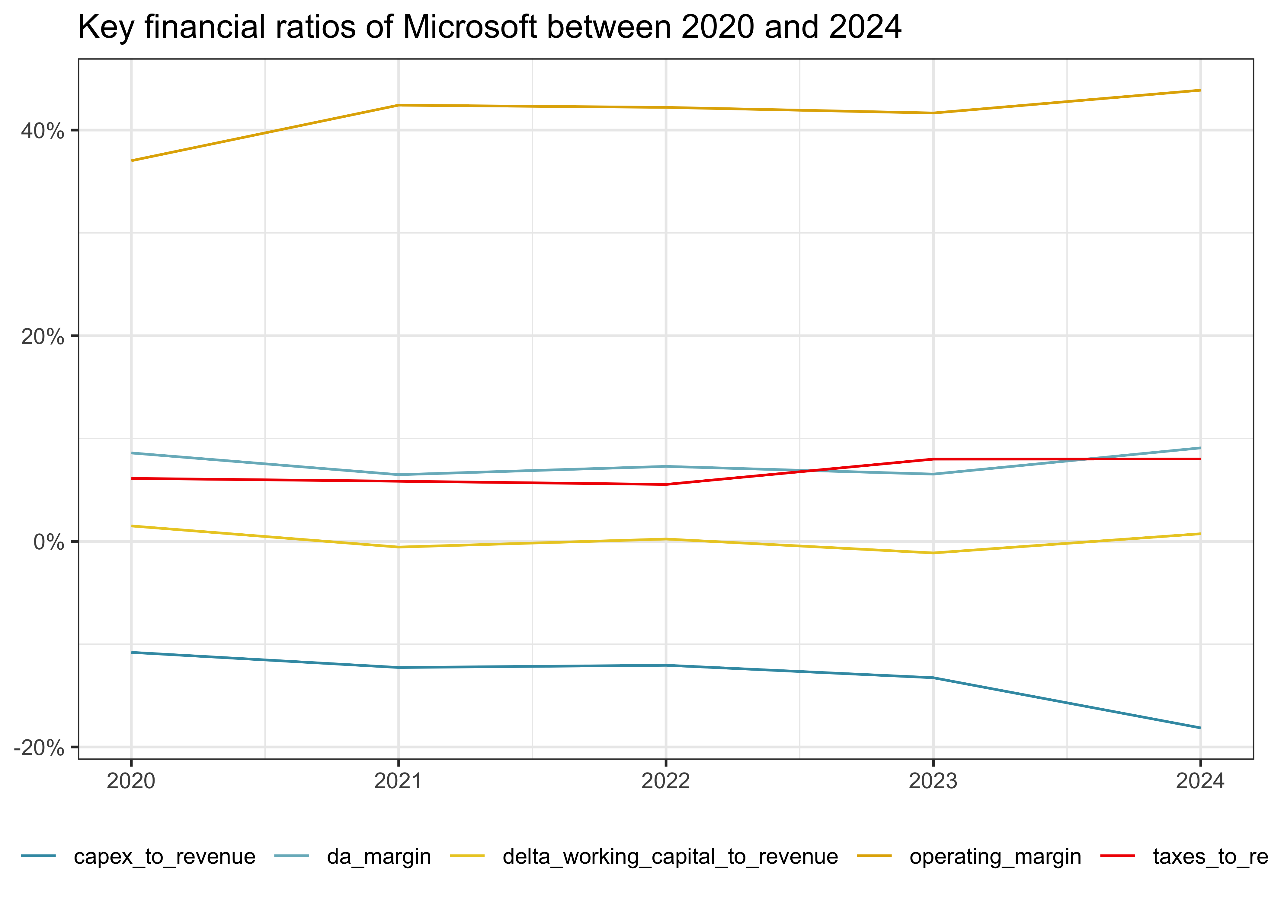
The operating margin, for instance, represents how much of each revenue dollar translates into operating profit (EBIT), while the CAPEX-to-revenue ratio indicates the company’s investment intensity.

For our DCF analysis, we need to project these ratios into the future. These projections should reflect both historical patterns and forward-looking considerations such as: Industry trends and competitive dynamics, company-specific growth initiatives, expected operational efficiency improvements, planned capital investments, or working capital management strategies. Overall, there is a lot to consider in practice. However, forecast ratios make this process tractable.

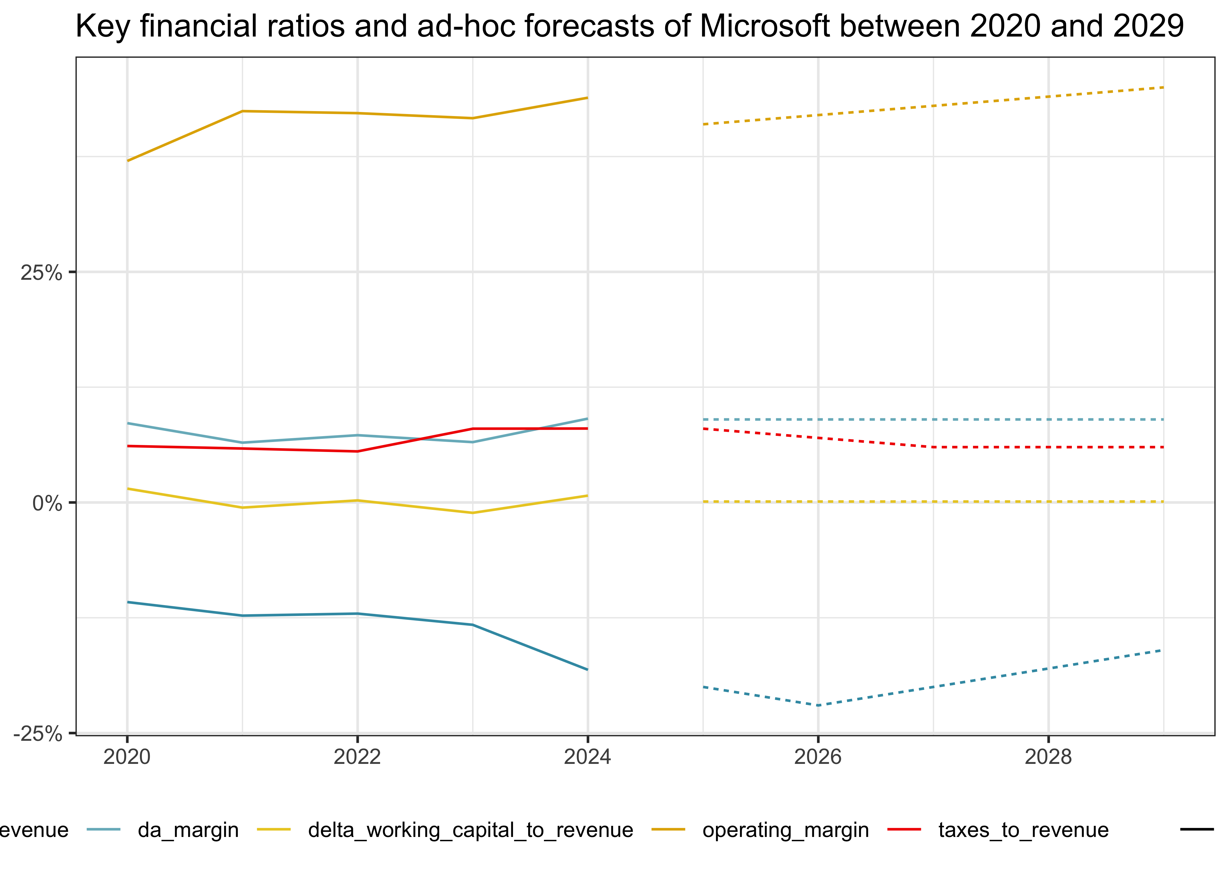
Another crucial question is the length of the forecast period. We use five years below ad-hoc, but you want to make detailed projections for each year when the company undergoes significant changes. As long as forecast ratios change, you need to make explicit forecasts. Once the company reaches a steady state, you can switch to computing the continuation value discussed later.

We demonstrate this forecasting approach in Figure 2. Note that our forecast ratio dynamics just serve as an example and are not grounded in deeper economic analysis.

dcf_data_forecast_ratios <- tribble(
  ~year, ~operating_margin, ~da_margin, ~taxes_to_revenue, ~delta_working_capital_to_revenue, ~capex_to_revenue,
  2025, 0.41, 0.09, 0.08, 0.001, -0.2,
  2026, 0.42, 0.09, 0.07, 0.001, -0.22,
  2027, 0.43, 0.09, 0.06, 0.001, -0.2,
  2028, 0.44, 0.09, 0.06, 0.001, -0.18,
  2029, 0.45, 0.09, 0.06, 0.001, -0.16
) |> 
  mutate(type = "Forecast")

dcf_data <- dcf_data |> 
  mutate(type = "Realized") |> 
  bind_rows(dcf_data_forecast_ratios)

dcf_data |> 
  pivot_longer(cols = c(operating_margin:capex_to_revenue)) |> 
  ggplot(aes(x = year, y = value, color = name, linetype = rev(type))) +
  geom_line() +
    scale_x_continuous(breaks = pretty_breaks()) +
  scale_y_continuous(labels = percent) +
  labs(
    x = NULL, y = NULL, color = NULL, linetype = NULL,
    title = "Key financial ratios and ad-hoc forecasts of Microsoft between 2020 and 2029"
  )

Figure 2: Historical ratios are based on financial statements provided through the FMP API, while forecasts are manually defined.

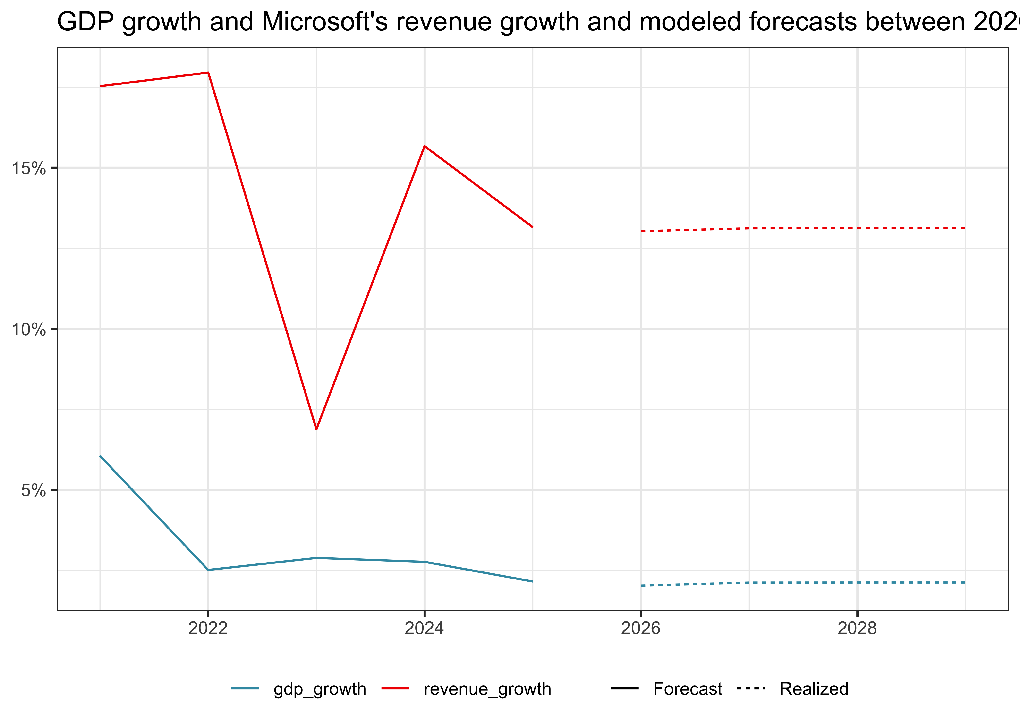
The final step in our FCF forecast is projecting revenue growth. While there are multiple approaches to this task, we demonstrate a GDP-based method that links company growth to macroeconomic forecasts.

We use GDP growth forecasts from the IMF World Economic Outlook (WEO) database as our baseline. The WEO provides comprehensive economic projections, though it is important to note that these forecasts are periodically revised as new data becomes available. We manually collect these forecasts and store them in a tibble.

gdp_growth <- tibble(
  year = 2020:2029,
  gdp_growth = c(-0.02163, 0.06055, 0.02512, 0.02887, 0.02765, 0.02153, 0.02028, 0.02120, 0.02122, 0.02122)
)

dcf_data <- dcf_data |> 
  left_join(gdp_growth, join_by(year))

Our approach models revenue growth as a linear function of GDP growth. This relation captures the intuition that company revenues often move in tandem with broader economic activity, though usually with different sensitivity. Let us estimate the model with historical data.

revenue_growth_model <- dcf_data |> 
  lm(revenue_growth ~ gdp_growth, data = _) |> 
  coefficients()
 
dcf_data <- dcf_data |> 
  mutate(
    revenue_growth_modeled = revenue_growth_model[1] + revenue_growth_model[2] * gdp_growth,
    revenue_growth = if_else(type == "Forecast", revenue_growth_modeled, revenue_growth)  
  ) 

The model estimates two parameters: (i) an intercept that captures the company’s baseline growth, and (ii) a slope coefficient that measures the company’s sensitivity to GDP changes. Then, we can use the model and the growth forecasts to make revenue growth projections. We visualize the historical and projected growth rates using this approach in Figure 3:

dcf_data |> 
  filter(year >= 2021) |> 
  pivot_longer(cols = c(revenue_growth, gdp_growth)) |> 
  ggplot(aes(x = year, y = value, color = name, linetype = rev(type))) +
  geom_line() +
  scale_x_continuous(breaks = pretty_breaks()) +
  scale_y_continuous(labels = percent) +
  labs(
    x = NULL, y = NULL, color = NULL, linetype = NULL,
    title = "GDP growth and Microsoft's revenue growth and modeled forecasts between 2020 and 2029"
  )

Figure 3: Realized revenue growth rates are based on financial statements provided through the FMP API, while forecasts are modeled unsing IMF WEO forecasts.

While more sophisticated approaches exist (e.g., proprietary analyst forecasts or bottom-up market analyses), this method provides a transparent and data-driven starting point for revenue projections.

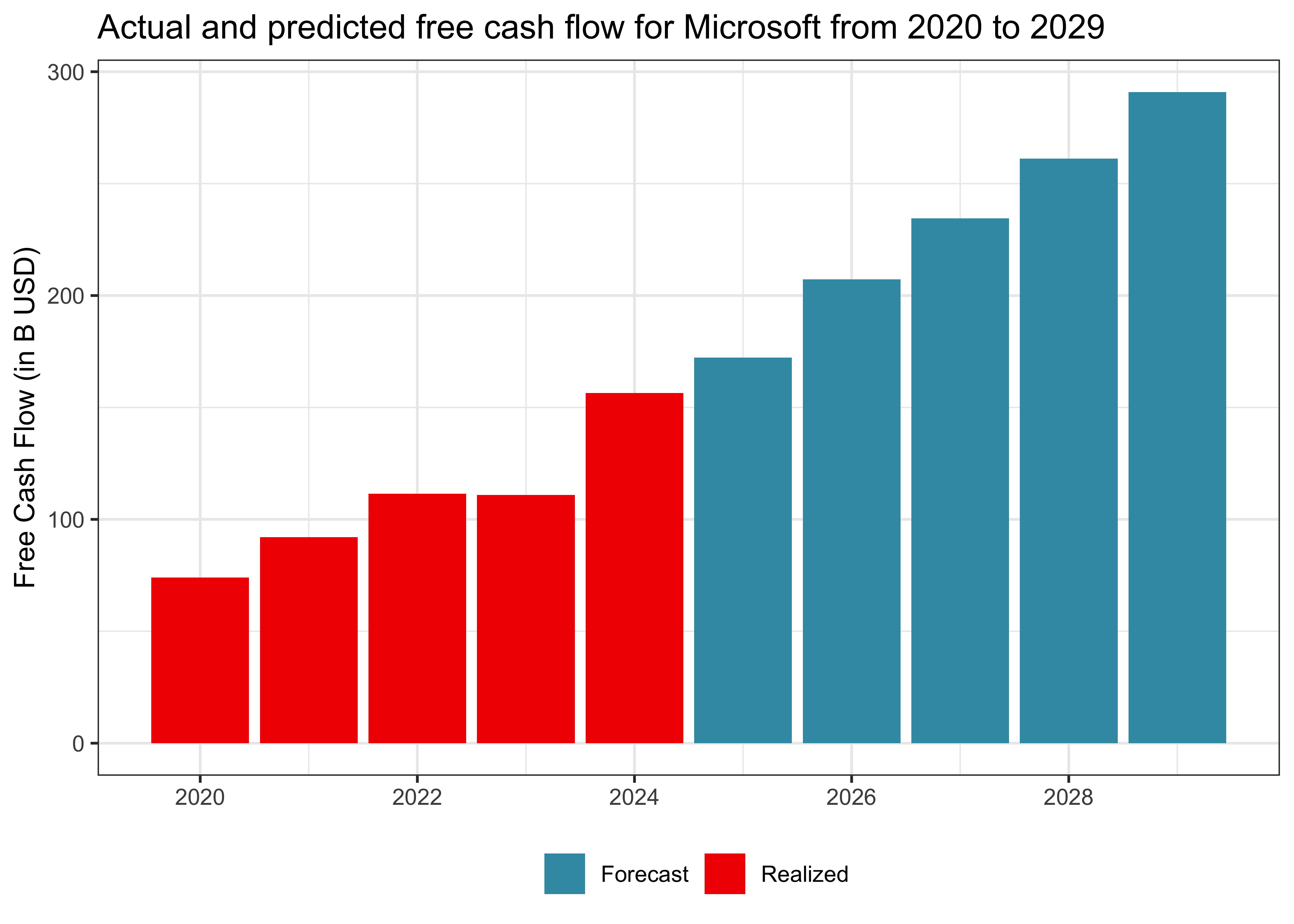
With all components in place - revenue growth projections and forecast ratios - we can now calculate our FCF forecasts. We must first convert our growth rates into revenue projections and then apply our forecast ratios to compute each FCF component.

dcf_data$revenue_growth[1] <- 0
dcf_data$revenue <- dcf_data$revenue[1] * cumprod(1 + dcf_data$revenue_growth)

dcf_data <- dcf_data |> 
  mutate(
    ebit = operating_margin * revenue,
    depreciation_and_amortization = da_margin * revenue,
    taxes = taxes_to_revenue * revenue,
    delta_working_capital = delta_working_capital_to_revenue * revenue,
    capex = capex_to_revenue * revenue,
    fcf = ebit + depreciation_and_amortization - taxes + delta_working_capital - capex
  )

We visualize the resulting FCF projections in Figure 4.

dcf_data |>
  ggplot(aes(x = year, y = fcf / 1e9)) +
  geom_col(aes(fill = type)) +
  scale_x_continuous(breaks = pretty_breaks()) +
  labs(
    x = NULL, y = "Free Cash Flow (in B USD)", fill = NULL,
    title = "Actual and predicted free cash flow for Microsoft from 2020 to 2029"
  )

Figure 4: Realized growth rates are based on financial statements provided through the FMP API, while forecasts are manually defined.

Continuation Value

A key component of DCF analysis is the continuation value (or terminal value), representing the company’s value beyond the explicit forecast period. This value often constitutes the majority of the total valuation, making its estimation particularly important. You can compute the continuation value once the company has reached its steady state.

The most common approach is the Perpetuity Growth Model (or Gordon Growth Model), which assumes FCF grows at a constant rate indefinitely. The formula for this model is:

\[TV_{T} = \frac{FCF_{T+1}}{r - g},\]

where \(TV_{T}\) is the terminal value at time \(T\), \(FCF_{T+1}\) is the free cash flow in the first year after our forecast period, \(r\) is the discount rate (typically WACC, see below), and \(g\) is the perpetual growth rate. A common mistake is to ignore the time shift in the model. You must compute \(FCF_{T+1}\), which is equal to \(FCF_{T}\cdot(1+g)\)

The perpetual growth rate \(g\) should reflect the long-term economic growth potential. A common benchmark is the long-term GDP growth rate, as few companies can sustainably grow faster than the overall economy indefinitely. Exceeding GDP growth indefinitely also implies that the whole economy eventually consists of one company. For example, the last 20 years of GDP growth is a sensible assumption (the nominal growth rate is 4% for the US).

Let us implement the Perpetuity Growth Model:

compute_terminal_value <- function(last_fcf, growth_rate, discount_rate){
  last_fcf * (1 + growth_rate) / (discount_rate - growth_rate)
}

last_fcf <- tail(dcf_data$fcf, 1)
terminal_value <- compute_terminal_value(last_fcf, 0.04, 0.08)
terminal_value / 1e9

[1] 7564

Note that while we use the Perpetuity Growth Model here, practitioners often cross-check their estimates with alternative methods like the exit multiple approach, which bases the terminal value on comparable company valuations.¹

Discount Rate

The final component of our DCF analysis involves discounting future cash flows to present value. We typically use the Weighted Average Cost of Capital (WACC) as the discount rate, representing the blended cost of financing for all company stakeholders. The WACC is the correct rate to discount cash flows distributed to both debt and equity holders, which is the case in our model as we use free cash flows.

The WACC formula combines the costs of equity and debt financing:

\[WACC = \frac{E}{D+E} \cdot r^E + \frac{D}{D+E} \cdot r^D \cdot (1 - \tau),\]

where \(E\) is the market value of the company’s equity with required return \(r^E\), \(D\) is the market value of the company’s debt with pre-tax return \(r^D\), and \(\tau\) is the tax rate.

While you can often find estimates of WACC from financial databases or analysts’ reports, you may need to calculate it yourself. Let us walk through the practical steps to estimate WACC using real-world data:

• \(E\) is typically measured as the market value of the company’s equity. One common approach is to use market capitalization from the stock exchange.
• \(D\) is often measured using the book value of the company’s debt. While this might not perfectly reflect market conditions, it is a practical starting point when market data is unavailable. Moreover, it is close to correct without default.
• The Capital Asset Pricing Model (CAPM) is a popular method to estimate the cost of equity \(r^E\). It considers the risk-free rate, the equity risk premium, and the company’s risk exposure (i.e., beta). For a detailed guide estimating the CAPM, we refer to Chapter Capital Asset Pricing Model.
• The return on debt \(r^D\) can also be estimated in different ways. For instance, effective interest rates can be calculated as the ratio of interest expense to total debt from financial statements. This gives you a real-world measure of what the company is currently paying. Alternatively, you can look up corporate bond spreads for companies in the same rating group.

If you would rather not estimate WACC manually, resources are available to help you find industry-specific discount rates. One of the most widely used sources is Aswath Damodaran’s database. He maintains an extensive database that provides a wealth of financial data, including estimated discount rates, cash flows, growth rates, multiples, and more. For example, if you are analyzing a company in the Computer Services sector, as we do here, you can look up the industry’s average WACC and use it as a benchmark for your analysis. The following code chunk downloads the WACC data and extracts the value for this industry:

library(readxl)

file <- tempfile(fileext = "xls")

url <- "https://pages.stern.nyu.edu/~adamodar/pc/datasets/wacc.xls"
download.file(url, file)
wacc_raw <- read_xls(file, sheet = 2, skip = 18)
unlink(file)

wacc <- wacc_raw |> 
  filter(`Industry Name` == "Computer Services") |> 
  pull(`Cost of Capital`)

Computing Enterprise Value

Having established all components, we can now compute the total company value (given that there are no non-operating activities). The enterprise value combines two elements:

• The present value of cash flows during the explicit forecast period and
• The present value of the continuation (or terminal) value.

This is expressed mathematically as:

\[ \text{Total DCF Value} = \sum_{t=1}^{T} \frac{\text{FCF}t}{(1 + \text{WACC})^t} + \frac{\text{TV}_{T}}{(1 + \text{WACC})^T}, \]

where \(T\) is the length of our forecast period. Let us implement this calculation in a simple function that takes the WACC and growth rate as input. Then, we present an example at the values discussed above.

compute_dcf <- function(wacc, growth_rate) {
  free_cash_flow <- dcf_data$fcf
  last_fcf <- tail(free_cash_flow, 1)
  terminal_value <- compute_terminal_value(last_fcf, growth_rate, wacc)
  
  years <- length(free_cash_flow)
  present_value_fcf <- free_cash_flow / (1 + wacc)^(1:years)
  present_value_tv <- terminal_value / (1 + wacc)^years
  total_dcf_value <- sum(present_value_fcf) + present_value_tv
  total_dcf_value
}

compute_dcf(wacc, 0.04) / 1e9

[1] 3781

Note that this valuation represents an enterprise value - the total value of the company’s operations. To arrive at the equity value, we need to subtract net debt (total debt minus cash and equivalents).

Sensitvity Analysis

DCF valuation is only as robust as its underlying assumptions. Given the inherent uncertainty in forecasting, it is crucial to understand how changes in key inputs affect our valuation.

While we could examine sensitivity to various inputs like operating margins or capital expenditure ratios, we focus on two critical drivers for our exposition:

• The perpetual growth rate, which determines long-term value creation and
• The WACC, which affects how we value future cash flows.

Let us implement a sensitivity analysis that varies these two parameters:

wacc_range <- seq(0.06, 0.08, by = 0.01)
growth_rate_range <- seq(0.02, 0.04, by = 0.01)

sensitivity <- expand_grid(
  wacc = wacc_range,
  growth_rate = growth_rate_range
) |>
  mutate(value = pmap_dbl(list(wacc, growth_rate), compute_dcf))

sensitivity |> 
  mutate(value = round(value / 1e9, 0)) |> 
  ggplot(aes(x = wacc, y = growth_rate, fill = value)) +
  geom_tile() +
  geom_text(aes(label = comma(value)), color = "white") +
  scale_x_continuous(labels = percent) + 
  scale_y_continuous(labels = percent) +
  scale_fill_continuous(labels = comma) + 
  labs(
    x = "WACC", y = "Perpetual growth rate", fill = "Enterprise value",
    title = "Enterprise value of Microsoft for different WACC and growth rate scenarios"
  ) + 
  guides(fill = guide_colorbar(barwidth = 15, barheight = 0.5))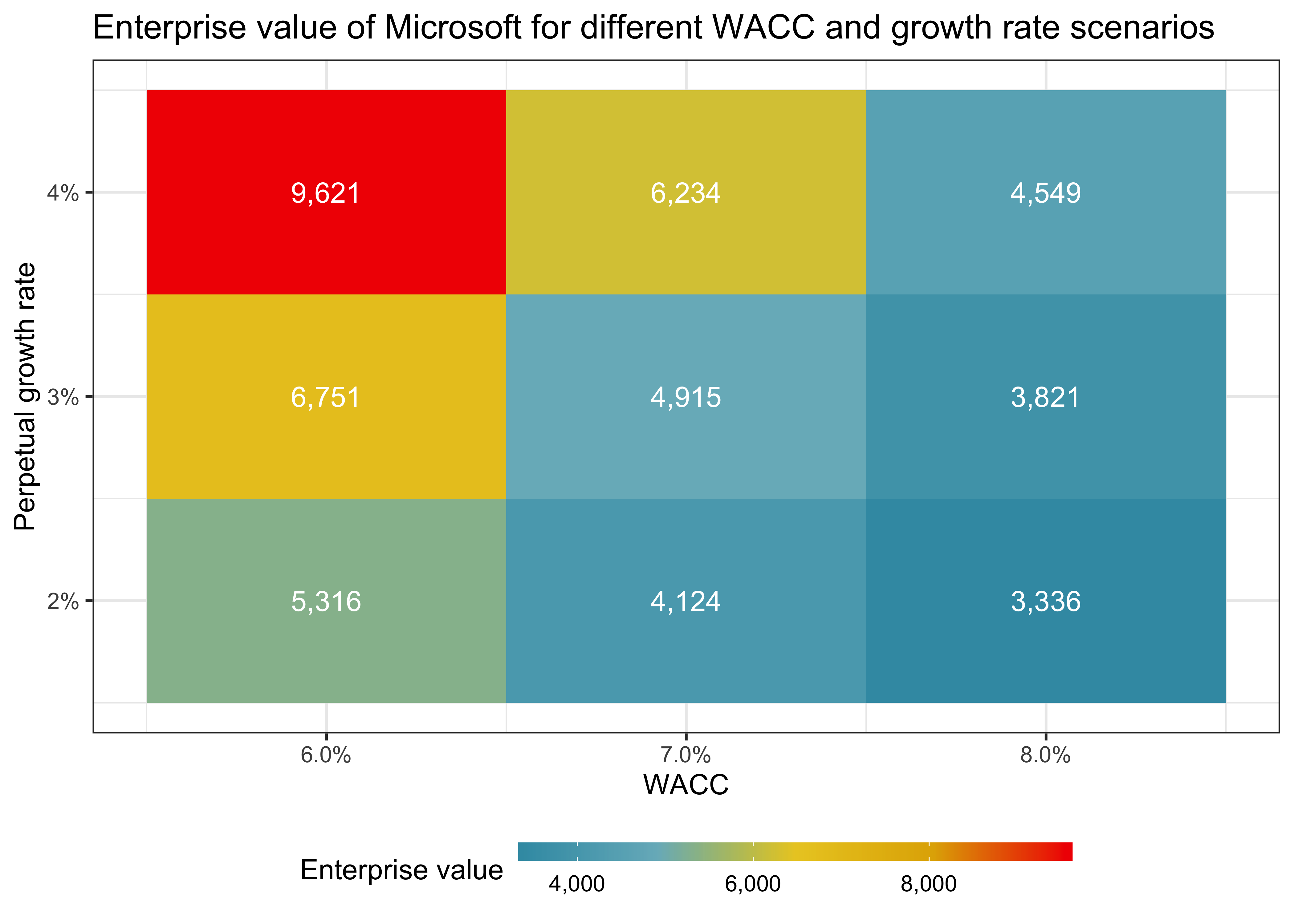

Figure 5: The enterprise values combine data from FMP API, ad-hoc forecasts of financial ratios, and IMF WEO growth forecasts.

Figure 5 reveals several key insights about our valuation: The valuation is highly sensitive to both WACC and growth assumptions, as small changes in either parameter can lead to substantial changes in enterprise value. Moreover, the relation between these parameters and company value is non-linear as the impact of growth rate changes becomes more pronounced at lower WACCs.

From Enterprise to Equity Value

As we have discussed, our DCF analysis yields the value of the company’s operations. We have assumed that there are no non-operating assets. Now, we explicitly consider their existence and show you how to compute the equity value belonging to shareholders.

Non-operating assets are not essential to operations but could, in some cases, generate income (e.g., marketable securities, vacant land, idle equipment). If they exist, you must restate the financial statements to exclude the impact of these non-operating assets. With their effects removed, you can conduct the DCF analysis presented above. Afterwards, you value these non-operating assets and add them to the DCF value to arrive at the company’s enterprise value.

Second, we want to discuss equity value. As you saw in the computation of the WACC, free cash flows go to both debt and equity holders. Hence, we must consider the share of the enterprise value that goes to debt. In theory, the value of debt is the market value of total debt, but in practice, typically book debt. This value has to be subtracted from enterprise value.

Combining these adjustments, we can compute the equity value that belongs to shareholders as:

\[\text{Equity Value} = \text{DCF Value} + \text{Non-Operating Assets} - \text{Value of Debt}\]

We leave it as an exercise to calculate the equity value using the DCF value from above.

Key takeaways

Discounted Cash Flow analysis provides a structured approach to company valuation. In this chapter, you learned to:

• Calculate free cash flow using financial statement data and ratio analysis.
• Project future cash flows by combining company-specific metrics with macroeconomic forecasts.
• Estimate terminal value using the perpetuity growth method.
• Apply appropriate discount rates based on industry benchmarks.
• Test the sensitivity of valuations to key assumptions.
• Convert enterprise values to equity values using balance sheet adjustments.

Exercises

1. Download financial statements for another company of your choice and compute its historical Free Cash Flow. Compare the results with the Microsoft example from this chapter.
2. Create a function that automatically generates FCF forecasts using different sets of ratio assumptions. Use it to create alternative scenarios for Microsoft.
3. Implement an exit multiple approach for terminal value calculation and compare the results with the perpetuity growth method.
4. Extend the sensitivity analysis to include operating margin assumptions. Create a visualization showing how changes in margins affect the final valuation.
5. Calculate Microsoft’s equity value by adjusting the CDF value as described above.

Footnotes

1. See (corporatefinanceinstitute.com/)[https://corporatefinanceinstitute.com/resources/valuation/exit-multiple/)] for an intuitive explanation of the exit multiple approach.